Assignment #1 - Deep Learning Fundamentals
Deep Learning / Spring 1398, Iran University of Science and Technology
Please pay attention to these notes:
- Assignment Due: 1397/12/24 23:59:00
- If you need any additional information, please review the assignment page on the course website.
- The items you need to answer are highlighted in red and the coding parts you need to implement are denoted by:
######################################## # Put your implementation here # ######################################## - We always recommend co-operation and discussion in groups for assignments. However, each student has to finish all the questions by him/herself. If our matching system identifies any sort of copying, you'll be responsible for consequences. So, please mention his/her name if you have a team-mate.
- Students who audit this course should submit their assignments like other students to be qualified for attending the rest of the sessions.
- Finding any sort of copying will zero down that assignment grade and also will be counted as two negative assignment for your final score.
- When you are ready to submit, please follow the instructions at the end of this notebook.
- If you have any questions about this assignment, feel free to drop us a line. You may also post your questions on the course Forum page.
- You must run this notebook on Google Colab platform, it depends on Google Colab VM for some of the depencecies.
- Before starting to work on the assignment Please fill your name in the next section AND Remember to RUN the cell.
Assignment Page: https://iust-deep-learning.github.io/972/assignments/01_deep_learning_fundamentals
Course Forum: https://groups.google.com/forum/#!forum/dl972/
Fill your information here & run the cell
#@title Enter your information & "RUN the cell!!" { run: "auto" }
student_id = 0 #@param {type:"integer"}
student_name = "" #@param {type:"string"}
Your_Github_account_Email = "" #@param {type:"string"}

print("your student id:", student_id)
print("your name:", student_name)


from pathlib import Path

ASSIGNMENT_PATH = Path('asg01')
ASSIGNMENT_PATH.mkdir(parents=True, exist_ok=True)
Classifying Persian Handwritten Digits
In class, we studied English handwritten digit classification problem using Keras framework and trained a neural network on the MNIST dataset. In this assignment, we would like to dig a little deeper and become more familiar with the implementation details, Keras features, and preprocessing stage in a deep-learning pipeline.
1 Preprocessing Stage
The preprocessing of the dataset is one of the most important and time-consuming steps of any deep learning project. Most of the time, we have a dataset that is not well-processed and ready to be fed into a neural network. Sometimes, the data might even be clean and organized, but not suitable to fit to our problem.
In this scenario, we have a dataset of Persian handwritten digits and we want to recognize digits only by looking at their image. Here is a brief stat of our dataset:
| Property | value |
|---|---|
| Resolution of samples | 200 dpi |
| Sample per each digit | ~10,000 samples |
| Training samples: | 60,000 samples |
| Test samples: | 20,000 samples |
First, let's download and explore our dataset. Run the following commands:
# Download the dataset
! wget -q http://iust-deep-learning.github.io/972/static_files/assignments/asg01_assets/data.zip

# Then, Extact it
! unzip data.zip -d .
Before going any further, we have to import some prerequisites:
import random
import numpy as np
import matplotlib.pyplot as plt
plt.rcParams['figure.figsize'] = (7,9) # Make the figures a bit bigger
import cv2
from keras.utils import to_categorical

from util import read_raw_dataset
Let's load the dataset using the provided function read_raw_dataset:
ds_images, ds_labels = read_raw_dataset("train.cdb")

print("Images:")
print(type(ds_images))
print(len(ds_images))
print(type(ds_images[0]))
print(ds_images[0].shape)

print("\nLabels:")
print(ds_labels[:30])
As you can see, train_images is a list of images and train_labels contains the labels for each element in the image list. Each image is represented as 2D (numpy) array of floats/ints.
So, lets look at some of the images:
# Randomly sample images, Re run the cell to see new images.
plt.figure(figsize=(12,8))
for i, index in enumerate(random.sample(list(range(len(ds_images))), 10)):
    plt.subplot(2,5,i+1)
    plt.imshow(ds_images[index], cmap='gray', interpolation='none')
    plt.title("Label {}".format(ds_labels[index]))
Pretty great! ha? But it seems images are not in a fixed dimension. Let's check our hypothesis:
unique_heights = list(set([m.shape[0] for m in ds_images]))
print("unique heights:", unique_heights)

unique_widths = list(set([m.shape[1] for m in ds_images]))
print("unique widths:", unique_widths)
Unfortunately, the images in our dataset do not have equal dimensions. So, we have to implement a function to fit the image in a fixed frame.
Note: There might be a situation where the image is bigger than the frame size; So, we first need to scale it down and then fit it into a fixed frame.
def fit_and_resize_image(src_image, dst_image_size):
  """
  fit the image in fixed size black background & resize it if needed.

  Args:
    src_image: 2d numpy array of image it may be in any shape
    dst_image_size: size of square background frame

  Returns:
    dst_image: 2d numpy array with shape (dst_image_size, dst_image_size). src_image should
               be fitted in the center of the background.

  Hint: OpenCv.resize, np.zeors may be useful for you.
  """

  ########################################
  #     Put your implementation here     #
  ########################################

  dst_image_width = dst_image_height

  src_image_height = src_image.shape[0]
  src_image_width = src_image.shape[1]

  if src_image_height > dst_image_height or src_image_width > dst_image_width:
      height_scale = dst_image_height / src_image_height
      width_scale = dst_image_width / src_image_width
      scale = min(height_scale, width_scale)
      img = cv2.resize(src=src_image, dsize=(0, 0), fx=scale, fy=scale, interpolation=cv2.INTER_CUBIC)
  else:
      img = src_image

  img_height = img.shape[0]
  img_width = img.shape[1]

  dst_image = np.zeros(shape=[dst_image_height, dst_image_width], dtype=np.uint8)

  y_offset = (dst_image_height - img_height) // 2
  x_offset = (dst_image_width - img_width) // 2

  dst_image[y_offset:y_offset+img_height, x_offset:x_offset+img_width] = img

  return dst_image
# Define a constant for our image size. please do not change it
IMAGE_SIZE = 32
Test your implementation using the following cell:
plt.subplot(1,2,1); plt.imshow(ds_images[10], cmap='gray', interpolation='none'); plt.title('Before')
plt.subplot(1,2,2); plt.imshow(fit_and_resize_image(ds_images[10], IMAGE_SIZE), cmap='gray', interpolation='none'); plt.title('After')
Congradulations! You've successfully implemented the fit_and_resize_image function. Now it's time to use that and create a function to read the dataset, process it, and return it as a Numpy array. As you may have noticed, image values are in the 0-255 range (0 is black and 255 is white). Generally, we first normalize our input when we want to feed them into a neural network. So, don't forget to normalize the images.
Note: When we're solving a multi-label classification probelm it is important for the labels to be in one-hot format. So remember to convert them to one-hot format before returning the function.
def read_dataset(dataset_path, images_size=32):
  """
  Read & process Persian handwritten digits dataset

  Args:
    dataset_path: path to dataset file
    image_size: size that should be fixed for all images.

  Returns:
    X: numpy ndarry with shape (num_samples, images_size, images_size) for normalized images
    y: numpy ndarry with shape (num_samples, 10) for labels in one-hot format
  """

  ########################################
  #     Put your implementation here     #
  ########################################

  images, labels = read_raw_dataset(dataset_path)

  X = np.zeros(shape=[len(images), images_size, images_size], dtype=np.float32)

  for i, img in enumerate(images):
    X[i] = fit_and_resize_image(img, IMAGE_SIZE) / 255.0

  Y = to_categorical(labels, num_classes=10, dtype=np.int)

  return X, Y
Question: Why should we normalize images to the [0-1] range?
$\color{red}{\text{Write you answer here}}$
Normalizing inputs make them have similar scales. This property will lead to a symmetric cost function, which is easier and faster to optimize.
To learn more watch this short video from Andew Ng: https://www.youtube.com/watch?v=FDCfw-YqWTE
Great! Now we have everything ready to build our neural network.
train_images, train_labels = read_dataset("train.cdb", IMAGE_SIZE)
test_images, test_labels = read_dataset("test.cdb", IMAGE_SIZE)

assert train_images.shape == (60000, IMAGE_SIZE, IMAGE_SIZE)
assert test_images.shape == (20000, IMAGE_SIZE, IMAGE_SIZE)

assert train_labels.shape == (60000, 10)
assert test_labels.shape == (20000, 10)

assert train_images.mean() > 0.0
assert test_images.mean() > 0.0

assert 0. <= train_images.min() and train_images.max() <= 1
assert 0. <= test_images.min() and test_images.max() <= 1
plt.figure(figsize=(10,8))
for i, index in enumerate(random.sample(list(range(len(train_images))), 6)):
    plt.subplot(2,3,i+1)
    plt.imshow(train_images[index], cmap='gray', interpolation='none')
    plt.title("Label {}".format(str(np.argmax(train_labels[index]))))
2 Building the model
In class, we exclusively used Keras Layers API to build a neural network; but, now, we want to get a little deeper and see what's going on behind this API.
2.1 Low level implementation
When we code in Keras, we are simply stacking up layer instances. However the implementation of neural networks is basically nothing but matrix multiplication and applying functions on them. Deep learning libraries are made to perform matrix multiplication in the first place; so, each of these frameworks should be equipped with matrix manipulation tools and APIs. Keras is no exception.
Perhaps you might think that Keras library has much higher level abstractions which makes significantly easier to work with. So, why do we have to learn low-level APIs? The point is that there are situations that we need low-level APIs. For example:
- Sometimes the layers we want to use are not included in the default Keras implementation thus we have to implement them by ourselves.
- More importantly, other deep learning frameworks such as Tensorflow and Pytorch are more commonly used in low-level mode. Learning such APIs will enable us to better understand the source codes of papers and existing projects available on the Internet.
Before starting to code, let's review some of the mathematics behind neural networks. We store connection's weights between layers in the shape of a matrix. Also, we represent layer bais as a matrix too. Here is an example:
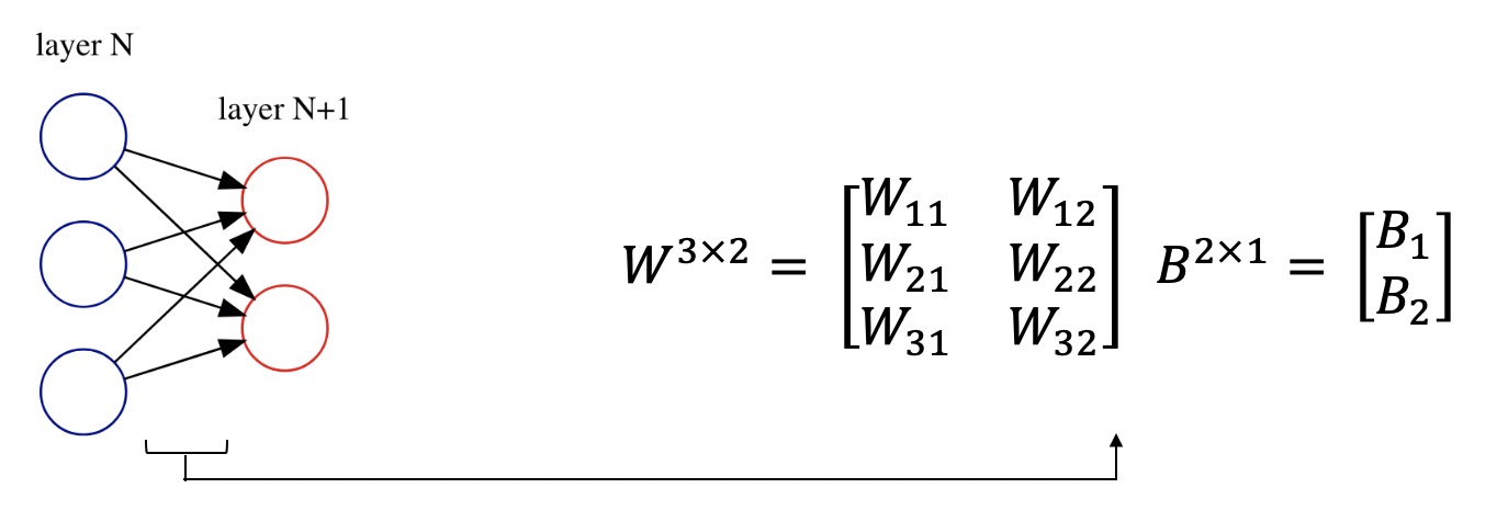
Suppose we have two layers in a neural network. Let $x \in \mathbb{R}^{N\times1}$ be the activations of the previous layer with $N$ nodes, $W$ be the weight of connections and $B$ be the bais for the current layer. Write an algebraic equation for the current layer with $M$ nodes and activations $h$. Also, specify dimensions of matrices $W, B, h$
$\color{red}{\text{Write you answer here}}$
$$ h = W^T . x + B \\ x \in \mathbb{R}^{N \times 1} \\ h \in \mathbb{R}^{M \times 1} \\ B \in \mathbb{R}^{M \times 1} \\ W \in \mathbb{R}^{N \times M} $$Please note that Broadcasting is used to calculate the sum of $W^T.x$ and $B$
But, computers, especially GPUs, are much more efficient in parallel computing. So, instead of feeding single input $\overrightarrow{x}$ through our neural network, why not feed them a batch? Thus, the input vector $\overrightarrow{x} \in \mathbb{R}^{N\times1}$ will be a matrix in the shape of $\mathbb{R}^{b \times N}$ ($b$ is the batch size) and each individual input will be one of $x$ rows.
Rewritre equation for $h$ above and specify the dimensions of matrices $W, B, h$
$\color{red}{\text{Write you answer here}}$
$$ h = x.W + B \\ x \in \mathbb{R}^{b \times N} \\ h \in \mathbb{R}^{b \times M} \\ B \in \mathbb{R}^{M \times 1} \\ W \in \mathbb{R}^{N \times M} $$Please note that Broadcasting is used to calculate the sum of $x.W$ and $B$
Let's import some prerequisites:
from keras import backend as K
from keras.layers import Layer, Dense, Dropout
from keras.models import Sequential
from keras.utils.layer_utils import count_params

from util import BaseModel
Here is the model class that we're going to implement. LowLevelMLP is a simple MLP network with a configurable number of hidden layers. To complete this section you need to fill its two methods __init__() and build_model(). We use __init__ to define networks weights and build_model() to specify operations between input and model weights to create the output.
Note: Using keras.layers is not allowed in this part. Please review keras documents for self.add_weight and K (Keras backend functions)
# Model configuration, Do not change
HIDDEN_LAYERS = [512, 128]
NUM_CLASSES = 10
NUM_EPOCH = 20
BATCH_SIZE = 512
class LowLevelMLP(BaseModel):

  def __init__(self, input_shape, hidden_layers, num_classes=10):
    """
    Initiate model with provided configuration
    Args:
      input_shape: size of input vector
      hidden_layers: a list of integer, specify num hidden layer node from left to right,
                     e.x.: [512, 128, ...]
      num_classes: an integer defining number of classes, this is the number of model ouput nodes
    """
    super(LowLevelMLP, self).__init__()

    self._input_shape = input_shape
    self._hidden_layers = hidden_layers
    self._num_classes = num_classes

    # Define model weights & biases according to self.hidden_layers and self.num_classes
    # To create weight you can use self.add_weight

    self._model_weights = []
    self._model_baiases = []

    ########################################
    #     Put your implementation here     #
    ########################################

    last_input_size = input_shape
    for h in self._hidden_layers + [num_classes]:
      self._model_weights.append(self.add_weight(
          name='hid_%s' % h,
          shape=(last_input_size, h),
          initializer='glorot_uniform'
      ))
      self._model_baiases.append(self.add_weight(
          name='bias_%s' % h,
          shape=(h, ),
          initializer='zeros'
      ))

      last_input_size = h


  def build_model(self, x):
    """
    The Model logic sits here.
    Args:
      x: an input tensor in shape of (?, input_size), ? is batch size and will be determined at the training phase
         e.x.: x is tensor with shape (?, 784) for the MNIST dataset

    Returns:
      pred: an output tensor with shape (?, self.num_classes)

    """

    # Define operations between input and model weights here
    # K.dot, K.relu, K.softmax might be useful for you.

    ########################################
    #     Put your implementation here     #
    ########################################

    h = x

    for w, b in zip(self._model_weights, self._model_baiases):
      h = K.relu(K.dot(h, w) + b)

    pred = K.softmax(h)

    return pred


ll_mlp = LowLevelMLP(IMAGE_SIZE ** 2, HIDDEN_LAYERS, NUM_CLASSES)
ll_mlp._model_weights, ll_mlp._model_baiases
assert  count_params(ll_mlp.trainable_weights) == sum(
    [(i*j) for i, j in zip([IMAGE_SIZE ** 2] + HIDDEN_LAYERS, HIDDEN_LAYERS + [NUM_CLASSES])]
    + HIDDEN_LAYERS
    + [NUM_CLASSES]
)
Let's train out model
# Before start training the model, we need to reshape the input so that each 32x32 image
# becomes a single 1024 dimensional vector.

x_train = train_images.reshape((-1, IMAGE_SIZE * IMAGE_SIZE))
y_train = train_labels.astype('float32')

x_test = test_images.reshape((-1, IMAGE_SIZE * IMAGE_SIZE))
y_test = test_labels.astype('float32')

print(x_train.shape, x_test.shape)
print(y_train.shape, y_test.shape)
ll_mlp.compile(optimizer='rmsprop', loss='categorical_crossentropy', metrics=['accuracy'])
ll_mlp_history = ll_mlp.fit(x_train, y_train, epochs=NUM_EPOCH, batch_size=BATCH_SIZE, validation_data=(x_test, y_test))
Now visualize the traning:
def visualize_loss_and_acc(history):
  history_dict = history.history
  loss_values = history_dict['loss']
  val_loss_values = history_dict['val_loss']
  acc = history_dict['acc']

  epochs = range(1, len(acc) + 1)

  f = plt.figure(figsize=(10,3))

  plt.subplot(1,2,1)
  plt.plot(epochs, loss_values, 'bo', label='Training loss')
  plt.plot(epochs, val_loss_values, 'b', label='Validation loss')
  plt.title('Training and validation loss')
  plt.xlabel('Epochs')
  plt.ylabel('Loss')
  plt.legend()


  acc_values = history_dict['acc']
  val_acc = history_dict['val_acc']

  plt.subplot(1,2,2)
  plt.plot(epochs, acc, 'bo', label='Training acc')
  plt.plot(epochs, val_acc, 'b', label='Validation acc')
  plt.title('Training and validation accuracy')
  plt.xlabel('Epochs')
  plt.ylabel('Loss')
  plt.legend()

  plt.show()
visualize_loss_and_acc(ll_mlp_history)
# Remember to run this cell after each time you update the model,
# this is one of deliverable items of your assignemnt
ll_mlp.save_weights(ASSIGNMENT_PATH / 'll_mlp.h5')
2.2 Custom Layer: Softmax
In this section, we're going to implement A custom Keras layer, A much realistic situation. For the sake of simplicity, we want to re-implement Softmax Layer. Before going through softmax implementation, let's review some of softmax details:
Softmax has an interesting property that is quite useful in practice, Softmax is invariant to constant offsets in the input, that is, for any input vector $x$ and any constant $c$,
$$ \mathrm{softmax(x) = softmax(x+c)} $$where $x + c$ means adding the constant c to every dimension of $x$. Remember that:
$$ softmax(x)_i = \dfrac{e^{x_i}}{\sum_{j} e^{x_j}} $$In practice, we make use of this property and choose $c = − max_i\ x_i$ when computing softmax probabilities for numerical stability (i.e., subtracting its maximum element from all elements of $x$).
class Softmax2D(Layer):
  """
  Softmax activation function, Only works for 2d arrays.
  """

  def __init__(self, **kwargs):
    super(Softmax2D, self).__init__(**kwargs)
    # We don't have any configuration for this custom layer,
    # But in future you should save any configuration related
    # to your layer in its constructor

  def compute_output_shape(self, input_shape):
    """Computes the output shape of the layer.

    Assumes that the layer will be built
    to match that input shape provided.

    Args:
      input_shape: Shape tuple (tuple of integers)
        or list of shape tuples (one per output tensor of the layer).
        Shape tuples can include None for free dimensions,
        instead of an integer.

    Returns:
      An input shape tuple.
    """
    # softmax of course doesn't change input shape,
    # so we can simply return input_shape as output shape
    return input_shape

  def build(self, input_shape):
    """
    This is where you will define your weights.
    This method must set self.built = True at the end,
    which can be done by calling super(Softmax2D, self).build().

    Args:
      input_shape: Keras tensor (future input to layer)
        or list/tuple of Keras tensors to reference
        for weight shape computations.
    """
    # As softmax is simple activation layer, we don't need any weight
    # definitions for this layer.
    super(Softmax2D, self).build(input_shape)

  def call(self, x):
    """
    This is where the layer's logic lives.

    Args:
      x: Input tensor, or list/tuple of input tensors.

    Returns:
      A tensor.
    """
    orig_shape = x.shape

    ########################################
    #     Put your implementation here     #
    ########################################

    x = x - K.max(x, axis=1, keepdims=True)
    x = K.exp(x)
    sum_vec = K.sum(x, axis=1, keepdims=True)
    x = x / sum_vec

    assert x.shape[1] == orig_shape[1] and len(x.shape) == len(orig_shape)
    return x
# Test your implementation
x = K.constant(np.array([[1001, 1002], [3, 4]]))
test2 = K.eval(Softmax2D()(x))
print(test2)
ans2 = np.array([
  [0.26894142, 0.73105858],
  [0.26894142, 0.73105858]])
assert np.allclose(test2, ans2, rtol=1e-05, atol=1e-06)
print("Passed!")
How to use our custom layer in practice?
# Create simple MLP network similar to what you implmented in previous section
s2d_mlp = Sequential()
s2d_mlp.add(Dense(512, activation='relu'))
s2d_mlp.add(Dense(128, activation='relu'))
s2d_mlp.add(Dense(NUM_CLASSES, activation=None))
s2d_mlp.add(Softmax2D()) # This is your custom layer,

# compile & train model
s2d_mlp.compile(optimizer='rmsprop', loss='categorical_crossentropy', metrics=['accuracy'])
s2d_history = s2d_mlp.fit(
    x_train, y_train,
    epochs=NUM_EPOCH,
    batch_size=BATCH_SIZE,
    validation_data=(x_test, y_test)
)
visualize_loss_and_acc(s2d_history)
# Remember to run this cell after each time you update the model,
# this is one of deliverable items of your assignemnt
s2d_mlp.save(str(ASSIGNMENT_PATH / 's2d_mlp.h5'))
3 Dropout
As you see, the validation error of the model starts to grow around epoch 5. But, our network is being optimized on the training loss during this time and its error is continuously reduced if the training dataset is not big enough (which is the case here). The model has mastered the task on the training set, but the learned network doesn't generalize to new examples that it has never seen!
Dropout is one of the most common regularization techniques used to prevent overfitting. It randomly shuts down some neurons in each iteration.
Question: Why Dropout helps model generalization (not overfitting)? What is the idea behind it? Explain with at least three reasons (feel free to use Google).
$\color{red}{\text{Write you answer here}}$
- Not all connections between neurons are really necessary! by using dropout we zero down some of them (in each iteration), forcing our model to learn data with less number of connections (or neurons) leading to a simpler model with higher generalization power.
- On the other hand, changing dropped neurons in each iteration makes our models an implicit ensemble of simpler neural networks, each learned the data in a different way. so we have many simple and diverse models which is expected to be better in generalization
- Also we can interpret dropout as adding noise in output layer of each layer. this can break up insignificant patterns that occur in each layer, which our network would tend to memorize in training without dropout.
[Thanks to Mohsen Tabassy for aggregating these reasons]
To learn more visit the following papers:
Improving IMDB sentiment classifier
Below is an MLP that is supposed to classify reviews in IMDB website as positive or negative (similar to what we saw in the class). But, this basic model starts to overfit very soon and, as a result, its performance on the validation set drops quickly. So, in this section, you need to improve this scenario. The following model is the base model; so, please do not change it. We will need it to compare our new model's performance.
from util import load_imdb_dataset
(x_train, y_train), (x_val, y_val), (x_test, y_test) = load_imdb_dataset()
imdb_mlp = Sequential()
imdb_mlp.add(Dense(16, activation='relu', input_shape=(10000,)))
imdb_mlp.add(Dense(16, activation='relu'))
imdb_mlp.add(Dense(1, activation='sigmoid'))

imdb_mlp.compile(optimizer='rmsprop',
              loss='binary_crossentropy',
              metrics=['acc'])

imdb_mlp_history = imdb_mlp.fit(x_train,
                                y_train,
                                epochs=20,
                                batch_size=512,
                                validation_data=(x_val, y_val))

print("Accuracy on Test set is:", imdb_mlp.evaluate(x_test, y_test)[1])
visualize_loss_and_acc(imdb_mlp_history)
As you can see, The model is overfitting quite fast! In this section you have to change the model, its prameters, and maybe add new layers to improve overfitting!
imdb_imprv = Sequential()

########################################
#     Put your implementation here     #
########################################

imdb_imprv.add(Dense(16, activation='relu'))
imdb_imprv.add(Dropout(0.5))                         # hidden layer dropout
imdb_imprv.add(Dense(16, activation='relu'))
imdb_imprv.add(Dropout(0.5))                         # hidden layer dropout
imdb_imprv.add(Dense(1, activation='sigmoid'))

imdb_imprv.compile(optimizer='rmsprop',
              loss='binary_crossentropy',
              metrics=['acc'])

imdb_imprv_history = imdb_imprv.fit(x_train,
                                y_train,
                                epochs=20,
                                batch_size=512,
                                validation_data=(x_val, y_val))

print("Accuracy on Test set is:", imdb_imprv.evaluate(x_test, y_test)[1])
Improved model:
visualize_loss_and_acc(imdb_imprv_history)
Base model:
visualize_loss_and_acc(imdb_mlp_history)
Question: Briefly explain why your changes improved model performance on the test set.
$\color{red}{\text{Write you answer here}}$
# Remember to run this cell after each time you update the model,
# this is one of deliverable items of your assignemnt
imdb_imprv.save(str(ASSIGNMENT_PATH / 'imdb_imprv.h5'))
References
- Khosravi, Hossein, and Ehsanollah Kabir. “Introducing a Very Large Dataset of Handwritten Farsi Digits and a Study on Their Varieties.” Pattern Recogn. Lett. 28, no. 10 (July 2007): 1133–1141. https://doi.org/10.1016/j.patrec.2006.12.022.
- Stanford Course: Deep Learning for NLP (CS224n)
- Coursera Course: Improving Deep Neural Networks: Hyperparameter tuning, Regularization and Optimization