Please pay attention to these notes:
- Assignment Due: 1398/01/10 23:59
- If you need any additional information, please review the assignment page on the course website.
- The items you need to answer are highlighted in red and the coding parts you need to implement are denoted by:
######################################## # Put your implementation here # ######################################## - We always recommend co-operation and discussion in groups for assignments. However, each student has to finish all the questions by him/herself. If our matching system identifies any sort of copying, you'll be responsible for consequences. So, please mention his/her name if you have a team-mate.
- Students who audit this course should submit their assignments like other students to be qualified for attending the rest of the sessions.
- Finding any sort of copying will zero down that assignment grade and also will be counted as two negative assignment for your final score.
- When you are ready to submit, please follow the instructions at the end of this notebook.
- If you have any questions about this assignment, feel free to drop us a line. You may also post your questions on the course Forum page.
- You must run this notebook on Google Colab platform, it depends on Google Colab VM for some of its depencecies.
- Before starting to work on the assignment Please fill your name in the next section AND Remember to RUN the cell.
Assignment Page: https://iust-deep-learning.github.io/972/assignments/02_tuning
Course Forum: https://groups.google.com/forum/#!forum/dl972/
Fill your information here & run the cell
#@title Enter your information & "RUN the cell!!" { run: "auto" }
student_id = 0 #@param {type:"integer"}
student_name = "" #@param {type:"string"}
Your_Github_account_Email = "" #@param {type:"string"}

print("your student id:", student_id)
print("your name:", student_name)


from pathlib import Path

ASSIGNMENT_PATH = Path('asg02')
ASSIGNMENT_PATH.mkdir(parents=True, exist_ok=True)
1. PlayOfTheGame
1.1 What is PUBG?
PlayerUnknown's Battlegrounds (PUBG) is a popular online survival multiplayer game. In this game, players are dropped into a wide, open area, and they must fight to the death using a variety of interesting weapons and vehicles while avoiding getting killed themselves. The last player or team standing wins the round. Although it's not necessary, but you can learn about other aspects of the game easily by searching the web, since the game is very popular and well known.
1.2 Kaggle competition - Can you predict the battle royale finish of PUBG Players?
Kaggle is a platform to compete with others in competitions which are based on machine learning tasks. Most of the time you are given some training and testing datasets for a specific task to build some good machine learning models.
In this assignment, you will participate in one of these competitions which is realted to PUBG. See this link for more details.
1.3 Data exploration and feature selection
Let's download the sampled dataset (100K)
! wget -q https://iust-deep-learning.github.io/972/static_files/assignments/asg02_assets/data.tar.gz
! tar xvfz data.tar.gz
Then, load the dataset
import pandas as pd

train = pd.read_csv('train.csv')
valid = pd.read_csv('valid.csv')

train.head()
As you can see, the training dataset consists of lots of different features for each instance, choose some arbitary numer of these features (at least three) which you think they are better for training. Explain how did you find them and why do you think this way?
$\color{red}{\text{Write your answer here}}$
</br> $\color{red}{\text{NOTE:}}$ Since the most important part in this assignment is the preprocessing and feature engineering, we concentrate on this part and leave the rest to the students (as the rest is implementing a simple feed forward MLP).
</br> There are several ways to select the most relevant features, here we share 3 feature selection techniques that are easy to use and also give good results:
1. Univariate Selection:
</br>
Some statistical tests can be used to select those features that have the strongest relationship with the output variable. The scikit-learn library provides the SelectKBest class that can be used with a suite of different statistical tests to select a specific number of features. You can find a compelete list of different offered statistical tests by SelectKBest class here. We used f_regression test here:
import pandas as pd
import numpy as np
from sklearn.feature_selection import SelectKBest
from sklearn.feature_selection import f_regression

pos_Numericals = ['assists', 'boosts', 'damageDealt',
              'DBNOs', 'headshotKills', 'heals',
              'killPlace','killPoints', 'kills',
              'killStreaks', 'longestKill',
              'matchDuration','maxPlace','numGroups',
              'revives','rideDistance','roadKills',
              'swimDistance', 'teamKills','vehicleDestroys',
              'walkDistance','weaponsAcquired','winPoints', 'winPlacePerc']


X = train[pos_Numericals].iloc[:,0:-2]
y = train[pos_Numericals].iloc[:,-1]

#apply SelectKBest class to extract top 3 best features
bestfeatures = SelectKBest(score_func=f_regression, k=3)
fit = bestfeatures.fit(X,y)
print(featureScores.nlargest(3,'Score'))  #print 3 best features
2.DT Feature Importance: </br> Decision trees score each feature based on their information gain (or other measures like Gini index). These scores can be used to select best features amongst all:
import pandas as pd
import numpy as np
from sklearn.tree import DecisionTreeRegressor
import matplotlib.pyplot as plt

pos_Numericals = ['assists', 'boosts', 'damageDealt',
              'DBNOs', 'headshotKills', 'heals',
              'killPlace','killPoints', 'kills',
              'killStreaks', 'longestKill',
              'matchDuration','maxPlace','numGroups',
              'revives','rideDistance','roadKills',
              'swimDistance', 'teamKills','vehicleDestroys',
              'walkDistance','weaponsAcquired','winPoints','winPlacePerc']


X = train[pos_Numericals].iloc[:,0:-2]
y = train[pos_Numericals].iloc[:,-1]

model = DecisionTreeRegressor()
model.fit(X,y)
#plot graph of feature importances for better visualization
feat_importances = pd.Series(model.feature_importances_, index=X.columns)
feat_importances.nlargest(10).plot(kind='barh')
plt.show()

3.Correlation Matrix with Heatmap: </br> Correlation states how the features are related to each other or the target variable.
import pandas as pd
import numpy as np
import seaborn as sns


pos_Numericals = ['assists', 'boosts', 'damageDealt',
              'DBNOs', 'headshotKills', 'heals',
              'killPlace','killPoints', 'kills',
              'killStreaks', 'longestKill',
              'matchDuration','maxPlace','numGroups',
              'revives','rideDistance','roadKills',
              'swimDistance', 'teamKills','vehicleDestroys',
              'walkDistance','weaponsAcquired','winPoints','winPlacePerc']

data  = train[pos_Numericals]

#get correlations of each features in dataset
corrmat = data.corr()
top_corr_features = corrmat.index
plt.figure(figsize=(15,15))
#plot heat map
g=sns.heatmap(data[top_corr_features].corr(),annot=True,cmap="RdYlGn")

As we can see the first technique suggests killPoints, rideDistance and walkDistance features, second one suggests walkDistance, killPlace and matchDuration and third one suggests walkDistance, killPlace and Boosts.
1.4 Implementation
Build and train a simple feed forward neural network regressor using your selected features to predict the desired outcome (player's final percentile rank). Choosing the number of layers, activasion functions, the optimizer, representation of input data and hyper parameters are completely up to you. Also feel free to add any new cells, functions, and classes if you want.
Import the dependencies
from keras.models import Sequential, load_model
Model Implementation
model = Sequential()

# Go on and use whatever MLP architecture you want
# Layers, and number of them is Totally up to you

########################################
#     Put your implementation here     #
########################################
Save the model to disk
# Remember to run this cell after each time you update the model,
# this is one of deliverable items of your assignemnt
model.save(str(ASSIGNMENT_PATH / 'potg.h5'))
1.5 Evaluation
In order to evaluate your model, we need you to fill the following function. Remember, all features are present in the input file, so you must choose your selected features, do all the requiered pre processing, feed your trained model with the result and finaly give us your predictions in a list.
Note: We'll run your model on a hidden test set using this function to measure its performance.
def predict(x):
  """
  Predict the placement of a player.

  Args:
    x (list[tuple()]): A list of players. Each player is a tuple(Id, groupId, matchId,
      assists, boosts, damageDealt, DBNOs, headshotKills, heals, killPlace, killPoints,
      kills, killStreaks, longestKill, matchDuration, matchType, maxPlace, numGroups,
      rankPoints, revives, rideDistance, roadKills, swimDistance, teamKills, vehicleDestroys,
      walkDistance, weaponsAcquired, winPoints)

  Returns:
    pred (list[float]): contains the placement prediction for each element in the input list.
      predictions are of 0-1 range where 1 corresponds to 1st place, and 0 corresponds
      to last place in the match
  """

  m = load_model(str(ASSIGNMENT_PATH / 'potg.h5'))
  pred = []

  # Do all of the preprocessing here,
  # you can use any combination of features you want.

  ########################################
  #     Put your implementation here     #
  ########################################

  assert isinstance(pred, list)
  assert len(pred) == len(x)
  assert all([isinstance(p, float) for p in pred])

  return pred
Notes
- The original train dataset has about 5 million records which is too large, but you can use our 100k sampled version which is provided for you and has almost the same distribuition as the original one.
- Since you are using a simple feedforward NN, your results don't have to be extraordinary! You will be graded in a comparative manner, so just try your best.
- There are lots of shared codes and ideas from other competitors for this challenge here. Feel free to take a look at these shared information, you can even get ideas and try them yourself, but be sure to not copy anything as copying has very serious consequences! You might even find similar implementations to what you have to do, but remember if you are able to find those implementations, so are we ;) .
2. Regularization
2.1 Underfitting and Overfitting, how to deal with them?
By using a neural network, we try to approximate a function for different purposes. In the training process, we want to maximize accuracy, while minimizing the error rate. However, there might be some problems with the model that we train.
One of the problems with deep neural networks is that they perform poorly in some cases. This poor performance might have different reasons. As you see in the pictures below, the problem might be due to the function we use, which might be too simple for such a task (underfitting) or too complex (overfitting).
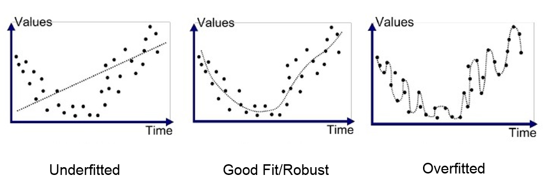
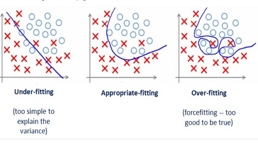
In the above pictures, the left graphs demonstrate an underfitted function that performs poorly on the task. This function has a high bias. On the other hand, the right graphs have a low bias and high variance. These are too-compilicated functions that have unnecessarily learned noisy details of the training set. To better understand this concept, let us explain what we mean by bias and variance.
Bias is the difference between the average prediction of our model and the correct value which we are trying to predict. Model with high bias pays very little attention to the training data and oversimplifies the model. It always leads to high error on training and test data.
Variance is the variability of model prediction for a given data point or a value which reflects the spread of our data. Model with high variance pays a lot of attention to training data and does not generalize on the data which it hasn’t seen before. As a result, such models perform very well on training data but have high error rates on test data.
In our models, we should try to balance the tradeoff between bias and variance so that the model can perform well on the test set. Overfitting is a more common problem in the training process and one way of recognizing it is by looking at the learning curves. In the below graph, the red curve is the validation error and the blue curve is the training error per each epoch of learning. The indication for the start of overfitting on the training set is that training error start to decline whereas the validation error increases.

2.2 How to overcome overfitting?
One way to overcome overfitting is through regularization. There are different regularization methods such as L2 or L1 regularization. In regularization, we add an extra term to the loss function of the neural network. This extra term could be L2 norm of weight matrices or their L1 norm. So, the cost function will be similar the following equation:
\begin{equation*} Cost function = Loss + \frac{\lambda}{ 2m} \sum_{i} \sum_{j} \left \lvert\lvert w_{i, j} \right \rvert\rvert^{2}_{F} \end{equation*}Instead of L2 norm, we can use L1 norm or a linear combination of each one. We can compute L1 norm and a linear combination of L1 and L2 norm using the following equations:
\begin{equation*} Cost function = Loss + \frac{\lambda}{ 2m} \sum_{i} \sum_{j} \left \lvert\lvert w_{i, j} \right \rvert\rvert \end{equation*}\begin{equation*} Cost function = Loss + \alpha( \frac{\lambda_{l2}}{ 2m} \sum_{i} \sum_{j} \left \lvert\lvert w_{i, j} \right \rvert\rvert^{2}_{F} ) + (1 - \alpha) (\frac{\lambda_{l1}}{ 2m} \sum_{i} \sum_{j} \left \lvert\lvert w_{i, j} \right \rvert\rvert ) \end{equation*}And $\alpha$ could be any real number between 0 and 1.
Adding the L1 norm to the cost function forces the weights to be close to zero, and this will lead to sparse weight matrices. This sparsity helps us to overcome the overfitting problem, because it limits the domain of possible values for weights and this prevents the function to be very compilicated.
2.3 How to use regularization methods in Keras?
In this assignment, we want to learn how to use regularization techniques in Keras and how they will affect weight matrices. In Keras, we can use regularizations for weight matrices, biases, and activations. To use regularization techniques, you should, for each layer, specify weather you want to use L1, L2, or a combination of them.
from keras import regularizers

Dense(64, kernel_regularizer=regularizers.l2(0.01), bias_regularizer=regularizers.l1(0.01), activity_regularizer=regularizers.l1_l2(l1=0.01, l2=0.01))
As you see in the above code, we can easily use the regularization techniques in each of the layers. You can set regularizer for weight matrix, bias vector, and activations of a layer by using the kernel_regularizer, bias_regularizer, activity_regularizer parameters, respectively. As you see, we used an L2 norm with $\lambda = 0.01$ to penalize the weight matrix, an L1 norm to penalize the bias vector, and a combination of L1 and L2 norms to penalize activations.
In Keras, we can also use other custom regularization approaches (which may not have been implemented in the framework). To implement and use a new regularization method, we should define a method like the following code and then pass it to the layer. In the following code, we implemented the L1 norm.
from keras import backend as K

def l1_reg(weight_matrix):
    return 0.01 * K.sum(K.abs(weight_matrix))

model.add(Dense(64, input_dim=64, kernel_regularizer=l1_reg))
Questions
We would like to train a neural network that learns to classify the data that in the following graph.
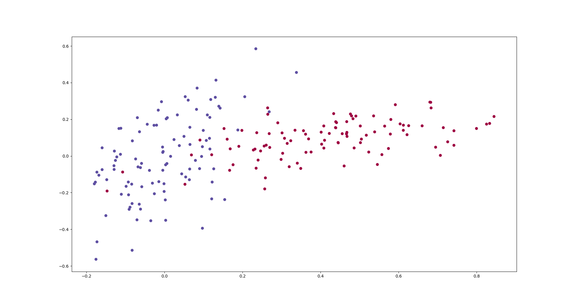
def get_data(nb_samples_per_class):
  mean = [0, 0]
  cov = [[.01, 0], [.014, 0.05]]
  x, y = np.random.multivariate_normal(mean, cov, nb_samples_per_class).T

  mean = [.4, .1]
  cov = [[0.01, .01], [.04, .01]]
  x1, y1 = np.random.multivariate_normal(mean, cov, nb_samples_per_class).T

  d1 = [[i, j, 1] for i, j in zip(x, y)]
  d2 = [[i, j, 0] for i, j in zip(x1, y1)]
  data = np.array(d1 + d2)
  np.random.shuffle(data)

  return data


data = get_data(100)

plt.scatter(data[:, 0], data[:, 1], c=data[:, 2].ravel(), cmap=plt.cm.Spectral)
plt.show()
Training
We trained the following model, and then, plotted the decision boundaries.
Decision boundaries have been presented in the following graph.
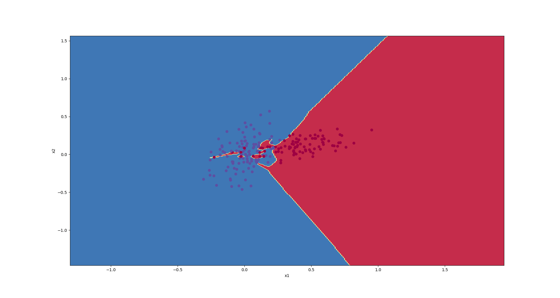
As you see, the approximated function is a very complex one that concentrates on the training set and cannot generalize well on the test test.
# For a single-input model with 2 classes (binary classification):

model = Sequential()
model.add(Dense(32, activation='relu', input_dim=2))
model.add(Dense(64, activation='relu'))
model.add(Dense(128, activation='relu'))
model.add(Dense(1, activation='sigmoid'))
model.compile(optimizer='rmsprop', loss='binary_crossentropy', metrics=['accuracy'])

# Train the model, iterating on the data in batches of 32 samples
val_data = get_data(30)
callback = model.fit(data[:, :2], data[:, 2], validation_data=(val_data[:, :2], val_data[:, 2]), epochs=2000, batch_size=32, verbose=0)
def plot_decision_boundary(model, X, y):
  y = np.around(y)
  # Set min and max values and give it some padding
  x_min, x_max = X[:, 0].min() - 1, X[:, 0].max() + 1
  y_min, y_max = X[:, 1].min() - 1, X[:, 1].max() + 1
  h = .01
  # Generate a grid of points with distance h between them
  xx, yy = np.meshgrid(np.arange(x_min, x_max, h), np.arange(y_min, y_max, h))
  # Predict the function value for the whole grid
  Z = np.around(model(np.c_[xx.ravel(), yy.ravel()]))
  Z = Z.reshape(xx.shape)

  # Plot the contour and training examples
  plt.contourf(xx, yy, Z, cmap=plt.cm.Spectral)
  plt.ylabel('x2')
  plt.xlabel('x1')
  plt.scatter(X[:, 0], X[:, 1], c=y.ravel(), cmap=plt.cm.Spectral)
  plt.show()

label = model.predict(data[:, :2])
plot_decision_boundary(lambda x : model.predict(x), data[:, :2], label)
model.fit() method returns a callback that contains history of the learning process. You can access the loss and accuracy of the model on training and validation sets in each epoch of learning.
callback.history['acc']
callback.history['loss']
callback.history['val_acc']
callback.history['val_loss']
Questions:
Note: In the following questions, whenever we mentioned learning curves, we mean three graphs. These three graphs indicate accuracy of model per epoch, error rate of the model per epoch, and the value of network loss for training, validation, and test sets.
Note: You can use plot_decision_boundary method to plot the decision boundaries.
Note: If learning curves oscillate, you can use moving average to smooth them. Use the following code.
def moving_avg(mist):
  N = 30
  cumsum, moving_aves = [0], []

  for i, x in enumerate(mlist, 1):
    cumsum.append(cumsum[i - 1] + x)
    if i >= N:
      moving_ave = (cumsum[i] - cumsum[i - N]) / N
      # can do stuff with moving_ave here
      moving_aves.append(moving_ave)
  return moving_aves
1) Plot learning curves and point out the approximate epoch that the model started to overfit on the data.
########################################
#     Put your implementation here     #
########################################

def plot_learning_curves(callbacks):

  plt.rcParams["figure.figsize"] = [20, 5]

  plt.subplot(1, 3, 1)
  for item in callbacks:
    callback = item['callback']
    model_name = item['model_name']
    plt.plot(moving_avg(callback.history['acc']), label='%s training' % model_name)
    plt.plot(moving_avg(callback.history['val_acc']), label='%s validation' % model_name)
  plt.title('accuracy')
  plt.legend()

  plt.subplot(1, 3, 2)
  for item in callbacks:
    callback = item['callback']
    model_name = item['model_name']
    plt.plot(moving_avg(callback.history['loss']), label='%s training' % model_name)
    plt.plot(moving_avg(callback.history['val_loss']), label='%s validation' % model_name)
  plt.title('loss')
  plt.legend()

  plt.subplot(1, 3, 3)
  for item in callbacks:
    callback = item['callback']
    model_name = item['model_name']
    training_error = [1-x for x in callback.history['acc']]
    validation_error = [1-x for x in callback.history['val_acc']]
    plt.plot(moving_avg(training_error), label='%s training' % model_name)
    plt.plot(moving_avg(validation_error), label='%s validation' % model_name)
  plt.title('error rate')
  plt.legend()
  plt.show()

plot_learning_curves([{'callback': callback, 'model_name': "overfitted"}])
It overfits on the epoch that the accuracy/loss/error of model on the trainning data start to incresase/decrease/deacrease, while the accuracy/loss/error of the model on validation data starts to fall/increase/increase.
2) Apply L1 and L2, separately, on all of the layers (just for weight matrices) and plot the learning curves and decision boundaries. Test it with three different values for $\lambda$ ($\lambda \in \{0.1, 0.01, 0.0001\} $). Which values work better? Why?
########################################
#     Put your implementation here     #
########################################

from keras import regularizers

def create_model_with_l1_on_weight(lambda_value):
  model1 = Sequential()
  model1.add(Dense(32, activation='relu', input_dim=2, kernel_regularizer=regularizers.l1(lambda_value)))
  model1.add(Dense(64, activation='relu', kernel_regularizer=regularizers.l1(lambda_value)))
  model1.add(Dense(128, activation='relu', kernel_regularizer=regularizers.l1(lambda_value)))
  model1.add(Dense(1, activation='sigmoid', kernel_regularizer=regularizers.l1(lambda_value)))
  model1.compile(optimizer='rmsprop', loss='binary_crossentropy', metrics=['accuracy'])

  callback1 = model1.fit(data[:, :2], data[:, 2], validation_data=(val_data[:, :2], val_data[:, 2]), epochs=2000, batch_size=32, verbose=0)
  return model, callback

def create_model_with_l2_on_weight(lambda_value):
  model1 = Sequential()
  model1.add(Dense(32, activation='relu', input_dim=2, kernel_regularizer=regularizers.l2(lambda_value)))
  model1.add(Dense(64, activation='relu', kernel_regularizer=regularizers.l2(lambda_value)))
  model1.add(Dense(128, activation='relu', kernel_regularizer=regularizers.l2(lambda_value)))
  model1.add(Dense(1, activation='sigmoid', kernel_regularizer=regularizers.l2(lambda_value)))
  model1.compile(optimizer='rmsprop', loss='binary_crossentropy', metrics=['accuracy'])

  callback1 = model1.fit(data[:, :2], data[:, 2], validation_data=(val_data[:, :2], val_data[:, 2]), epochs=2000, batch_size=32, verbose=0)
  return model, callback

def create_model_with_l1_on_bias(lambda_value):
  model1 = Sequential()
  model1.add(Dense(32, activation='relu', input_dim=2, bias_regularizer=regularizers.l1(lambda_value)))
  model1.add(Dense(64, activation='relu', bias_regularizer=regularizers.l1(lambda_value)))
  model1.add(Dense(128, activation='relu', bias_regularizer=regularizers.l1(lambda_value)))
  model1.add(Dense(1, activation='sigmoid', bias_regularizer=regularizers.l1(lambda_value)))
  model1.compile(optimizer='rmsprop', loss='binary_crossentropy', metrics=['accuracy'])

  callback1 = model1.fit(data[:, :2], data[:, 2], validation_data=(val_data[:, :2], val_data[:, 2]), epochs=2000, batch_size=32, verbose=0)
  return model, callback

def create_model_with_l2_on_bias(lambda_value):
  model1 = Sequential()
  model1.add(Dense(32, activation='relu', input_dim=2, bias_regularizer=regularizers.l2(lambda_value)))
  model1.add(Dense(64, activation='relu', bias_regularizer=regularizers.l2(lambda_value)))
  model1.add(Dense(128, activation='relu', bias_regularizer=regularizers.l2(lambda_value)))
  model1.add(Dense(1, activation='sigmoid', bias_regularizer=regularizers.l2(lambda_value)))
  model1.compile(optimizer='rmsprop', loss='binary_crossentropy', metrics=['accuracy'])

  callback1 = model1.fit(data[:, :2], data[:, 2], validation_data=(val_data[:, :2], val_data[:, 2]), epochs=2000, batch_size=32, verbose=0)
  return model, callback
########################################
#     Put your implementation here     #
########################################

model, callback1 = create_model_with_l1_on_weight(0.1)
model, callback01 = create_model_with_l1_on_weight(0.1)
model, callback0001 = create_model_with_l1_on_weight(0.0001)
plot_learning_curves([{'callback': callback1, 'model_name': "l1 lambda = 0.1"},
                      {'callback': callback01, 'model_name': "l1 lambda = 0.01"},
                      {'callback': callback0001, 'model_name': "l1 lambda = 0.0001"}])


model, callback1 = create_model_with_l2_on_weight(0.1)
model, callback01 = create_model_with_l2_on_weight(0.1)
model, callback0001 = create_model_with_l2_on_weight(0.0001)
plot_learning_curves([{'callback': callback1, 'model_name': "l2 lambda = 0.1"},
                      {'callback': callback01, 'model_name': "l2 lambda = 0.01"},
                      {'callback': callback0001, 'model_name': "l2 lambda = 0.0001"}])
$\color{red}{\text{Write you answer here}}$
Lambda = 0.0001 would be a better option for both of the regularization methods. Lambda = 0.1 or 0.01 might result low loss but high error rate because it forces most of the weight to be zero inorder to reduce the cost function.
3) Now, apply the L1 and L2 on biases and compare with the result of last question (compare each $\lambda$ separately). Which one works better? Why?
########################################
#     Put your implementation here     #
########################################

########################################
#     Put your implementation here     #
########################################
model, callbackw = create_model_with_l1_on_weight(0.1)
model, callbackb = create_model_with_l1_on_bias(0.1)
plot_learning_curves([{'callback': callbackw, 'model_name': "l1 on weight"},
                      {'callback': callbackb, 'model_name': "l1 on bias"}])

model, callbackw = create_model_with_l1_on_weight(0.01)
model, callbackb = create_model_with_l1_on_bias(0.01)
plot_learning_curves([{'callback': callbackw, 'model_name': "l1 on weight"},
                      {'callback': callbackb, 'model_name': "l1 on bias"}])

model, callbackw = create_model_with_l1_on_weight(0.0001)
model, callbackb = create_model_with_l1_on_bias(0.0001)
plot_learning_curves([{'callback': callbackw, 'model_name': "l1 on weight"},
                      {'callback': callbackb, 'model_name': "l1 on bias"}])


model, callbackw = create_model_with_l2_on_weight(0.1)
model, callbackb = create_model_with_l2_on_bias(0.1)
plot_learning_curves([{'callback': callbackw, 'model_name': "l2 on weight"},
                      {'callback': callbackb, 'model_name': "l2 on bias"}])

model, callbackw = create_model_with_l2_on_weight(0.01)
model, callbackb = create_model_with_l2_on_bias(0.01)
plot_learning_curves([{'callback': callbackw, 'model_name': "l2 on weight"},
                      {'callback': callbackb, 'model_name': "l2 on bias"}])

model, callbackw = create_model_with_l2_on_weight(0.0001)
model, callbackb = create_model_with_l2_on_bias(0.0001)
plot_learning_curves([{'callback': callbackw, 'model_name': "l2 on weight"},
                      {'callback': callbackb, 'model_name': "l2 on bias"}])
$\color{red}{\text{Write you answer here}}$
Addidn regularization on weights work better than biases because they have less impact on the output of each layer; In theory, you can assume that biases are zero, and it would work.
4) Implement a linear combination of L1 and L2 norm and test it for three different value of $\alpha$ ($\alpha \in \{0.3, 0.5, 0.7\} $).
########################################
#     Put your implementation here     #
########################################

from keras import backend as K


def custom_reg(alpha, lambda1=0.001, lambda2=0.001):
  def l1_l2(weight_matrix):
      return alpha * lambda2 * K.sum(K.square(weight_matrix)) + (1 - alpha) * lambda1 * K.sum(K.abs(weight_matrix))
  return l1_l2

def create_model_with_custom_regularization(alpha):
  model1 = Sequential()
  model1.add(Dense(32, activation='relu', input_dim=2, kernel_regularizer=custom_reg(alpha)))
  model1.add(Dense(64, activation='relu', kernel_regularizer=custom_reg(alpha)))
  model1.add(Dense(128, activation='relu', kernel_regularizer=custom_reg(alpha)))
  model1.add(Dense(1, activation='sigmoid', kernel_regularizer=custom_reg(alpha)))
  model1.compile(optimizer='rmsprop', loss='binary_crossentropy', metrics=['accuracy'])

  callback1 = model1.fit(data[:, :2], data[:, 2], validation_data=(val_data[:, :2], val_data[:, 2]), epochs=2000, batch_size=32, verbose=0)
5) Compare the results of questions 2 and 4 for each value of $\alpha$ separately (one plot for each value of $\alpha$ that contains learning curves for L1, L2, and linear combination of them). $\lambda = 0.01$
model, callbacka1 = create_model_with_custom_regularization(0.3)
model, callbacka2 = create_model_with_custom_regularization(0.5)
model, callbacka3 = create_model_with_custom_regularization(0.7)
plot_learning_curves([{'callback': callbacka1, 'model_name': "custom alpha = 0.3"},
                      {'callback': callbacka2, 'model_name': "custom alpha = 0.5"},
                      {'callback': callbacka3, 'model_name': "custom alpha = 0.5"}
                     ])
$\color{red}{\text{Write you answer here}}$
linear combination of L1 and L2 would be a better option than L1 because it will make L1 more stable.
6) Try to prevent the overfitting by adding the regularization term to each layer of the network, and then, plot the decision boundaries and learning curves. Add each of the regularization techniques seperatly and compare them with eachother. $\lambda = 0.01$
########################################
#     Put your implementation here     #
########################################

lambda1 = 0.001

modelf1 = Sequential()
modelf1.add(Dense(32, activation='relu', input_dim=2, kernel_regularizer=regularizers.l2(lambda1)))
modelf1.add(Dense(64, activation='relu', kernel_regularizer=regularizers.l2(lambda1)))
modelf1.add(Dense(128, activation='relu'))
modelf1.add(Dense(1, activation='sigmoid'))
modelf1.compile(optimizer='rmsprop', loss='binary_crossentropy', metrics=['accuracy'])

callbackf1 = modelf1.fit(data[:, :2], data[:, 2], validation_data=(val_data[:, :2], val_data[:, 2]), epochs=2000, batch_size=32, verbose=0)

modelf2 = Sequential()
modelf2.add(Dense(32, activation='relu', input_dim=2, kernel_regularizer=regularizers.l2(lambda1)))
modelf2.add(Dense(64, activation='relu'))
modelf2.add(Dense(128, activation='relu', kernel_regularizer=regularizers.l2(lambda1)))
modelf2.add(Dense(1, activation='sigmoid'))
modelf2.compile(optimizer='rmsprop', loss='binary_crossentropy', metrics=['accuracy'])

callbackf2 = modelf1.fit(data[:, :2], data[:, 2], validation_data=(val_data[:, :2], val_data[:, 2]), epochs=2000, batch_size=32, verbose=0)

lambda1 = 0.001

modelf3 = Sequential()
modelf3.add(Dense(32, activation='relu', input_dim=2, kernel_regularizer=regularizers.l2(lambda1)))
modelf3.add(Dense(64, activation='relu'))
modelf3.add(Dense(128, activation='relu'))
modelf3.add(Dense(1, activation='sigmoid', kernel_regularizer=regularizers.l2(lambda1)))
modelf3.compile(optimizer='rmsprop', loss='binary_crossentropy', metrics=['accuracy'])

callbackf3 = modelf1.fit(data[:, :2], data[:, 2], validation_data=(val_data[:, :2], val_data[:, 2]), epochs=2000, batch_size=32, verbose=0)

plot_learning_curves([{'callback': callbackaf1, 'model_name': "layer 1"},
                      {'callback': callbackaf2, 'model_name': "layer 2"},
                      {'callback': callbackaf3, 'model_name': "layer 3"}
                     ])
7) Run you implemented code for question 2 with $\lambda = 0.01$ multiple times. Which regularization technique is stable? (By stable, we mean a model that prevents the overfitting all the time)
########################################
#     Put your implementation here     #
########################################
$\color{red}{\text{Write you answer here}}$
L2 is more stable than L1
3. Optimizers
Run the following block to import requirements
%matplotlib inline
import numpy as np
import keras
import keras.backend as K
from keras import optimizers
from keras.models import Model
from keras.layers import Input, Dense
import matplotlib.pyplot as plt
import matplotlib.animation as animation
plt.ioff()
Part 1: Minimizing a custom function
Consider this structure: a smiple model with a single node in input layer and a single node in output dense layer (with use_bias argument set to False). This way, if we set the input to the constant value 1, the output will always be equal to the single weight variable between the input node and the output node.
Using this technique, we can define a custom arbitary function and find its minimum value using predefined optimizer methods in keras.
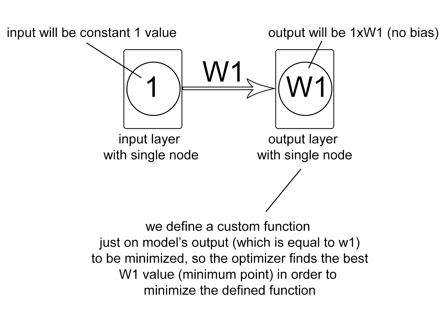
See the following code for better underestanding:
def minimize (config):

  '''
  The wrapper function which makes
  the custom fucntion suitable for
  model.compile method
  '''
  def custom_loss(layer):

    '''
    custom function:
    f(x) = ((x-1)^2)*(x+1)*(x^2-3)*(x-4)/90
    Notice that y_pred value is exactly
    equal to our single weight value as
    explained before. Also Notice that
    y_ture value dosn't actually play
    any rule in defined function, but
    it needs to be passed.
    '''
    def loss(y_true,y_pred):
      # in order to change objective function, this line must be changed
      return ((y_pred-1)**2)*(y_pred+1)*(y_pred**2-3)*(y_pred-4)/90.0

    return loss


  # Creating single input single output model
  init_vals = config['init_vals']
  inp = Input(shape=(1,))
  weights = Dense(1, use_bias=False)
  out = weights(inp)
  model = Model (inputs=inp, outputs=out)
  weights.set_weights([np.array([init_vals])])
  model.compile (optimizer=config['optimizer'], loss=custom_loss(out))


  # Storing w1 (our single weight) values
  # during training for later plotting.
  w1_history = [init_vals[0]]
  for epoch in range(config['epochs']):
    # Notice the constant 1 input value.
    # Also Notice that the output value
    # passed to fit method dosn't really
    # matter, however it can not be None
    # and needs to be passed.
    model.fit (x=[1.0], y=[1.0], epochs= 1, verbose=0);
    w1_history.append (weights.get_weights()[0][0][0])

  return w1_history
Part 2: Visualising
Using this piece of code, we can visualize the optimizer's steps for minimizing the objective function.
def visualize(independent_variable_history):
  fig = plt.figure(figsize = (4,4))

  X = np.linspace(-2.1, 4.1, 200)

  '''
  @@ in order to change objective function, this line
  must be changed
  '''
  Y = ((X-1)**2)*(X+1)*(X**2-3)*(X-4)/90.0

  def ani(coords):
    plt.cla()
    plt.plot(X, Y, "b")
    return plt.plot([coords[0]],[coords[1]], 'go')

  def frames():
      for x in independent_variable_history:
          '''
          @@ in order to change objective function, this line
          must be changed
          '''
          yield x, ((x-1)**2)*(x+1)*(x**2-3)*(x-4)/90.0

  from IPython.display import HTML
  return HTML(animation.FuncAnimation(fig, ani, frames=frames, interval=30).to_jshtml())
You can use these codes by passing a configuration dictionary like this:
config = {
    "init_vals": [-2.0],
    "optimizer": optimizers.SGD(lr=0.1, decay=1e-6, momentum=0.9),
    "epochs" : 200
}
independent_variable_history = minimize(config)
visualize(independent_variable_history)
Part 3: Your part
- A) In the previous proposed technique, we had only a single independent variable (the single weight of the model). Expand this idea in a way that supports more than one independent variable, explain your toughts.
$\color{red}{\text{Write you answer here}}$ </br> This can be achieved esaily by using 2 (or more) output nodes instead of one, the rest is similar.
- B) Change the optimizer config values in order to make the model fall in the other local minima.
#### FIRST LOCAL MINIMUM

config = {
    "init_vals": [-2.0],
    "optimizer": optimizers.SGD(lr= 0.1 , decay= 1e-6 , momentum= 0.8),
    "epochs" : 200
}
independent_variable_history = minimize(config)
visualize(independent_variable_history)
#### SECOND LOCAL MINIMUM

config = {
    "init_vals": [-2.0],
    "optimizer": optimizers.SGD(lr= 0.13 , decay= 1e-6 , momentum= 0.83),
    "epochs" : 200
}
independent_variable_history = minimize(config)
visualize(independent_variable_history)
- C) Explain how does each of SGD configuration parameters affect the behaviour of optmizer.
$\color{red}{\text{Write you answer here}}$ </br>
Learning rate: gradinet descent can only determine the direction towards the local minimum but does not give us any information about the step size we should take, learning rate is our step size towards this direction. so if we choose it too big the algorithem may not converge and if we choose it too small it might result in a super slow convergence.
Decay: this parameter reduces learning rate per iteration.
Momentum: with Stochastic Gradient Descent we don’t compute the exact derivate of our loss function. Instead, we’re estimating it on a small batch. Which means we’re not always going in the optimal direction, because our derivatives are ‘noisy’. So, we use a weighted average of current calculated gradient and the previous one to have a better estimate which is closer to the actual derivate than our noisy calculations. the Momentum parameter is the mentioned weight value in the weighted average calculation, with higher values of this parameter the average is closer to the previous gradient vector rather than the new one. Increasing this parameter is kind of like making the path more slippery, which helps passing through local minima.
- D) Checkout Adam optimizer in keras documentation. Use Adam optimizer instead of SGD. Try different parameter configurations and see the effects. Based on your observations, explain how does each of these parameters affect the behaviour of Adam optimizer.
$\color{red}{\text{Write you answer here}}$
- Learning rate and Decay parameters are similar to SGD.
- $\beta_1$ and $\beta_2$: Adam optimizer uses the following update rules:
$g_i$ is th gradient vector at step $i$. The ${\beta_1}$ parameter is obviously similar to momentum in SGD. </br> In this equations, $v$ is called uncentered variance and it kind of represents how certain we are about the direction of calculated noisy gradient. In the original paper the fraction $ \frac {m_i}{\sqrt{v_i}}$ is called signal to noise ratio (SNE). Consider a situation in which the direction of the gradient vector is changing alot, in this situation $m$ becomes smaller and smaller (since the gradients do not follow any particular direction, their mean becomes approximately zero) but uncentered variance becomes larger and larger and in this situation the SNE becomes near zero, so the weight changes become smaller since we are not sure about the direction. On the other hand, consider a situation in which the calculated gradeint does not change alot and almost always is the same. In this situation we are sure about the direction, uncentered variance becomes approximately equal to $m^2$ and SNE becomes one. </br> ${\beta_2}$ is the control parameter in computing the moving average of $v$. In most situations the default value (0.999) works fine. We refer you to the original paper for the mathematical details.
- E) In which situations do you think using Adam optimizer would be more effective than regular SGD optimizer? Explain your reasons.
$\color{red}{\text{Write you answer here}}$ </br> As Adam uses a modified step size for each parameter, in most cases using it results in a much faster convergence than SGD, however in practice, in few cases it makes the model overfitted. There is no general rule about when to use Adam over SGD, it most certainly depends on the problem, but Adam is a very good first choice in most situations.
References
- Kaggle competition PUBG Finish Placement Prediction