Please pay attention to these notes:
- Assignment Due: 1398/03/17 23:59
- If you need any additional information, please review the assignment page on the course website.
- The items you need to answer are highlighted in red and the coding parts you need to implement are denoted by:
######################################## # Put your implementation here # ######################################## - We always recommend co-operation and discussion in groups for assignments. However, each student has to finish all the questions by him/herself. If our matching system identifies any sort of copying, you'll be responsible for consequences. So, please mention his/her name if you have a team-mate.
- Students who audit this course should submit their assignments like other students to be qualified for attending the rest of the sessions.
- Finding any sort of copying will zero down that assignment grade and also will be counted as two negative assignment for your final score.
- When you are ready to submit, please follow the instructions at the end of this notebook.
- If you have any questions about this assignment, feel free to drop us a line. You may also post your questions on the course's forum page.
- You must run this notebook on Google Colab platform; there are some dependencies to Google Colab VM for some of the libraries.
- Before starting to work on the assignment please fill your name in the next section AND Remember to RUN the cell.
Assignment Page: https://iust-deep-learning.github.io/972/assignments/04_nlp_intro
Course Forum: https://groups.google.com/forum/#!forum/dl972/
Fill your information here & run the cell
#@title Enter your information & "RUN the cell!!"
student_id = 0 #@param {type:"integer"}
student_name = "" #@param {type:"string"}
Your_Github_account_Email = "" #@param {type:"string"}

print("your student id:", student_id)
print("your name:", student_name)


from pathlib import Path

ASSIGNMENT_PATH = Path('asg04')
ASSIGNMENT_PATH.mkdir(parents=True, exist_ok=True)
1. Word2vec
In any NLP task with neural networks involved, we need a numerical representation of our input (which are mainly words). A naive solution would be to use a huge one-hot vector with the same size as our vocabulary, each element representing one word. But this sparse representation is a poor usage of a huge multidimentional space as it does not contain any usefull information about the meaning and semantics of a word. This is where word embedding comes in handy.
1.1 What is word embedding?
Embeddings are another way of representing vocabulary in a lower dimentional (compared to one-hot representation) continuous space. The goal is to have similar vectors for the words with similar meanings (so the elements of the vector actually carry some information about the meaning of the words). The question is, how are we going to achieve such representations? The idea is simple but elegant: The words appearing in the same context are likely to have similar meanings.
So how can we use this idea to learn word vectors?
1.2 How to train?
We are going to train a simple neural network with a single hidden layer to perform a certain task, but then we’re not actually going to use that neural network for the task we trained it on! Instead, the goal is actually just to learn the weights of the hidden layer and use this hidden layer as our word representation vector.
So lets talk about this "fake" task. We’re going to train the neural network to do the following: given a specific word (the input word), the network is going to tell us the probability for every word in our vocabulary of being near to this given word (be one of its context words). So the network is going to look somthing like this (considering that our vocabulary size is 10000):
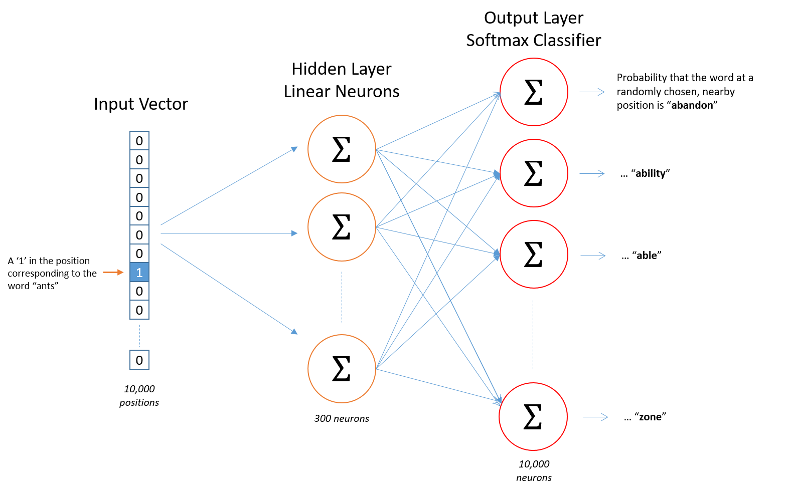
By training the network on this task, the words which appear in similar contexts are forced to have similar values in the hidden layer since they are going to give similar outputs, so we can use this hidden layer values as our word representation.
- This approach is called skip-gram. There is another similar but slightly different approach called CBOW. Read about CBOW and explain its general idea:
$\color{red}{\text{Write your answer here}}$ </br> CBOW is very similar to skip-gram, the difference is in the task we are training our model on. In skip-gram we ask model for the context words given the center word, but in CBOW we ask model for the center word given context words! Skip-gram works well with small amount of the training data and represents well even rare words or phrases. On the other hand CBOW is several times faster to train than the skip-gram and has slightly better accuracy for the frequent words.
1.3 A practical challenge with softmax activation
Softmax is a very handy tool when it comes to probability distribution prediction problems, but it has its downsides when the number of the nodes grows too large. Let's look at softmax activation in our output layer:
$$ \mathbf{S_{ij}} = \frac {e^{W_{j}^T Y_{i-1}}}{\sum_{j=1}^{N} e^{W_{j}^T Y_{i-1}}\ } \ $$As you can see, every single output is dependent on the other outputs, so in order to compute the derivative with respect to any weight, all the other weights play a role! For a 10000 output size this results in milions of mathematical operations for a single weight update, which is not practical at all!
- There are various techniques to solve this issue, like using hierarchical softmax or NCE (Noise Contrastive Estimation). The original Word2vec paper proposes a technique called Negative sampling. Read about this technique and explain its general idea:
$\color{red}{\text{Write your answer here}}$
</br>
Recall that the desired ouput was consisting of some few number of 1 values (the words in the context) and lots of 0 values (other irrelevant words), in other words with each training sample, we were trying to make the embedding vectors of our target word and the context words become closer while making our target embedding and all irrelevant word embeddings become less similar. This is actually the main issue, because using all irrelevant words is unnecessary, causing soft max activation computations be too heavy. Negative sampling is one of the ways of addressing this problem with just selecting a couple of irrelevant words at random (instead of all). The end result is that for example if cat appears in the context of food, then the vector of food is more similar to the vector of cat than the vectors of several other randomly chosen words (e.g. democracy, greed, Freddy), instead of all other words in language. This makes word2vec much much faster to train.
- Explain why is it called Negative sampling? What are these Negative samples?
$\color{red}{\text{Write your answer here}}$ </br> These randomly choosen irrelevant words are called Negative samples and they are called this way because we are trying to seprate their embeddings from our target word's.
1.4 Word2vec in code
There is a very good library called gensim for using word2vec in python. You can train your own word vectors on your own corpora or use available pretrained models. For example the following model is word vectors for a vocabulary of 3 million words and phrases trained on roughly 100 billion words from a Google News dataset with vector length of 300 features:
!wget -c "https://s3.amazonaws.com/dl4j-distribution/GoogleNews-vectors-negative300.bin.gz"
!gunzip GoogleNews-vectors-negative300.bin.gz
Lets load this model in python:
import gensim

# Load Google's pre-trained Word2Vec model.
model = gensim.models.KeyedVectors.load_word2vec_format('GoogleNews-vectors-negative300.bin', binary=True)

print ("# of words", len(model.vocab))
print ("# of vectors", len(model.vectors))
print ("the first 10 elements of embedding vector for the word king:",
       model.vectors[model.vocab["king"].index][:10])
As you can see it requires a huge amount of memory!
- Use gensim library, find the 3 most similar words to each given following target word using similar_by_word method, find all these words embeddings, reduce their dimension to 2 using a dimension reduction algorithm (eg. t-SNE or PCA) and plot the results in a 2d-scatterplot:
target_words = ["king", "horse", "blue", "apple",
                "computer", "lion", "rome", "tehran",
                "orange", "red", "army", "cat",
                "asia", "mouse"]


########################################
#     Put your implementation here     #
########################################
similars = []

for word in target_words:
  s = (model.similar_by_word(word, 3))
  for w in s:
    similars.append(w[0])

target_words += similars

vectors = []
for word in target_words:
  vectors.append(model.vectors[model.vocab[word].index])

from sklearn.manifold import TSNE
import numpy as np
import matplotlib.pyplot as plt

tsne = TSNE(n_components=2).fit_transform (np.array(vectors))

for i,t in enumerate(target_words):
    x = tsne[i,0]
    y = tsne[i,1]
    plt.plot(x, y, marker='x', color='red')
    plt.text(x+0.3, y+0.3, t, fontsize=9)

plt.show()

You can find the cosine similarity between two word vectors using similarity method:
print ('logitech', '/', 'cat', '->', model.similarity('logitech', 'cat'))
print ('black', '/', 'criminal', '->', model.similarity('black', 'criminal'))
print ('white', '/', 'criminal', '->', model.similarity('white', 'criminal'))
print ('black', '/', 'offensive', '->', model.similarity('black', 'offensive'))
print ('white', '/', 'offensive', '->', model.similarity('white', 'offensive'))
- As you can see there is a meaningfull similarity between the word logitech (a provider company of personal computer and mobile peripherals) and the word cat, even though they shouldn't have this much similarity. Explain why do you think this happens? Find more examples for this phenomenon.
$\color{red}{\text{Write your answer here}}$
</br>
This phenomenon is one of the most important current research trends in the field of word sense disambiguation. The problem occurs when there are two words with the same spellings but different meanings. For example in this case, the word mouse causes the problem. Since Logitech company is a computer peripherals provider, it is likely to appear in the same context as the word mouse (meaning a computer I/O device). On the other hand the words cat and mouse (meaning an animal) are likely to appear in the same context too. The result is the embeddings of words Logitech and cat being close to eachother because of the word mouse. More examples:
print ('steel', '/', 'cloth', '->', model.similarity('steel', 'cloth'))         # because of iron
print ('ipod', '/', 'banana', '->', model.similarity('ipod', 'banana'))      # because of apple
- It seems that words like criminal and offensive are more similar to the word black rather than white. It is claimed that word2vec model trained on Google News suffers from gender, racial and religious biases. Explain why do you think this happens and find 4 more examples:
$\color{red}{\text{Write your answer here}}$ </br> This happens because any bias in the articles that make up the Word2vec corpus is inevitably captured in the geometry of the vector space. As a matter of fact the model does not learn anything unless we teach it! This type of biases happen because the training set is biased in this way (e.g. the news about dark skinned people doing crime are more covered.
########################################
#     Put your implementation here     #
########################################

print ('islam', '/', 'terrorism', '->', model.similarity('islam', 'terrorism'))
print ('christianity', '/', 'terrorism', '->', model.similarity('christianity', 'terrorism'))
print ("------")
print ('kurdish', '/', 'rebellion', '->', model.similarity('kurdish', 'rebellion'))
print ('turkish', '/', 'rebellion', '->', model.similarity('turkish', 'rebellion'))
print ("------")
print('poor', '/', 'black', '->', model.similarity('poor', 'black'))
print('poor', '/', 'white', '->', model.similarity('poor', 'white'))
print ("------")
print('villain','/'  'iran', '->', model.similarity('villain', 'iran'))
print('villain','/'  'ameriaca', '->', model.similarity('villain', 'usa'))
print ("------")
Word vectors have some other cool properties, for example we know the relation between the meanings of the two words "man" and "woman" is similar to the relation between words "king" and "queen". So we expect $e_{queen} - e_{king} = e_{women} - e_{man}$ or $e_{queen} = e_{king} + e_{women} - e_{man}$ .
- Show whether the above equation holds or not by following these steps:
- Extract the embedding vectors for these words.
- Subtract the vector of "man" from vector of "woman" and add the vector of "king"
- Find the cosine similarity of the resulting vector with the vector for the word "queen"
########################################
#     Put your implementation here     #
########################################

man, woman = model['man'], model['woman']
king, queen = model['king'], model['queen']

print ("similarity of e_queen with e_king + e_woman - e_man : ", model.cosine_similarities(woman-man+king, [queen])[0])
2. Context representation using a window-based neural network
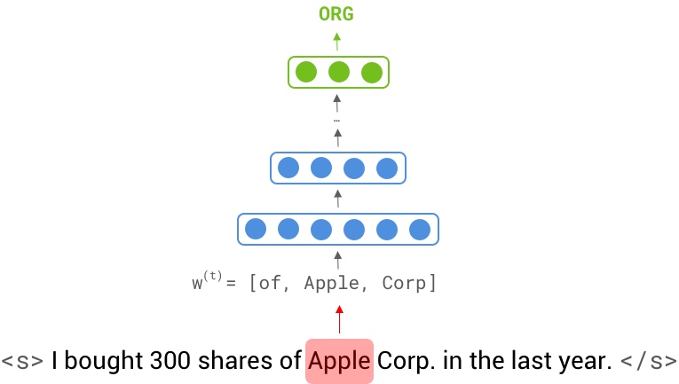
From the previous section, we saw that word vectors can store a lot of semantic information in themselves. But can we solve an NLP task by just feeding them through a simple neural network? Assume we want to find all named entities in a given sentence (aka Named Entity recognition). For example, In "I bought 300 shares of Apple Corp. in the last year". We want to locate the word "Apple" and categorize it as an Organization entity.
Obviously, a neural network cannot guess the type entirely based on a single word. We need to provide an extra piece of information to help the decision. This piece of information is called "Context" . We can decide if the word Apple is referring to the company or fruit by seeing it in a sentence (context). However, feeding a complete sentence through a network is inefficient as it makes the input layer really big even for a 10-word sentence (10 * 300 = 3000, assuming an embedding size of 300).
To make training such network possible, we make the input only by including K surrounding neighbor words. hence, apple can be easily classified as a company by looking at the context window [ the, apple, corporation ]
In a window-based classifier, every input sentence $X = [\mathbf{x^{(1)}}, ... , \mathbf{x^{(T)}}]$ with a label sequence $Y = [\mathbf{y^{(1)}}, ..., \mathbf{y^{(T)}}]$ is split into $T$ <context window, center word label> data points. We create a context window $\mathbf{w^{(t)}}$ for every token $\mathbf{x^{(t)}}$ in the original sentence by concatenating its k surrounding neighbors: $\mathbf{w^{(t)}} = [\mathbf{x^{(t-k)}}; ...; \mathbf{x^{(t)}}; ...; \mathbf{x^{(t+k)}}]$, therefore our new data point is created as $\langle \mathbf{w^{(t)}} , \mathbf{y^{(t)}} \rangle$.
Having word case information might also help the neural network to find name entities with higher confidence. To incorporate casing, every token $\mathbf{x^{(t)}}$ is augmented with feature vector $\mathbf{c}$ representing such information: $\mathbf{x^{(t)}} = [\mathbf{e^{(t)}};\mathbf{c^{(t)}}]$ where $\mathbf{e^{(t)}}$ is the corresponding embedding.
In this section, we aim to build a window based feedforward neural network on the NER task, and then analyze its limitations through a case study.
Let's import some depencecies.
! wget -q https://iust-deep-learning.github.io/972/static_files/assignments/asg04_assets/data.tar.gz
! tar xvfz data.tar.gz > /dev/null

from IPython.display import SVG
from pprint import pprint
import numpy as np
import keras
from keras.models import Model
from keras.utils.vis_utils import model_to_dot
from keras.utils import to_categorical

from ner_util import read_dataset, convert_to_window_based, preprocess, LBLS, \
      UNK_TOK, plot_confusion_matrix, visualize_loss_and_acc, print_sentence
from ag_news_util import read_ag_news, AG_NEWS_LBLS, create_model_input, create_vocab

! pip install -q tqdm flair
from tqdm import tqdm
from flair.data import Sentence
from flair.models import SequenceTagger
And define the model's hyperparameters:
NUM_NEIGHBORS = 1
WINDOW_SIZE = 2 * NUM_NEIGHBORS + 1
VOCAB_SIZE = 10*1000
EMBEDDING_DIM = 300
NUM_CLASSES = 5
BATCH_SIZE = 512
2.1 Preprocessing
As discussed earlier, we want to include the word casing information. Here's our desired function to encode the casing detail in d-dimensional vector. Words "Hello", "hello", "HELLO" and "hELLO" have four different casings. Your encoding should support all of them; In other words, the implemented function must return 4 different vectors for these inputs, but the same output for "Bye" and "Hello", "bye" and "hello", "bYe" and "hEllo", etc.
# The Default dimension for the casing vector.
# You can change it to match your desiered encoding.
CASING_DIM = 4

CASES = ["xx", "XX", "Xx", "xX"]
case2id = {c: i for i, c in enumerate(CASES)}

def get_casing(word):
  """
  Return the casing information in a numpy array.

  Args:
    word(str): input word, E.g. Hello

  Returns:
    np.array(shape=(CASING_DIM,)): encoded casing

  Hint: You might find the one-hot encoding useful.
  """
  casing = np.zeros(shape=(CASING_DIM,))

  ########################################
  #     Put your implementation here     #
  ########################################

  # all lowercase
  if word.islower():
    case = "xx"
  # all uppercase
  elif word.isupper():
    case = "XX"
  # starts with capital
  elif word[0].isupper():
    case = "Xx"
  # has non-initial capital
  else:
    case = "xX"

  casing = to_categorical(case2id[case], len(CASES))

  assert casing.shape == (CASING_DIM,)
  return casing

print("case(hello) =", get_casing('hello'))
print("case(Hello) =", get_casing('Hello'))
print("case(HELLO) =", get_casing('HELLO'))
print("case(hEllO) =", get_casing('hEllO'))
Describe two other features that would help the window-based model to perform better (apart from word casing).
$\color{red}{\text{Write your answer here}}$
- POS Tags (e.g. Verb, Adj)
- NER Tag of previous token
CONLL 2003[1] is a classic NER dataset; It has five tags per each word: [PER, ORG, LOC, MISC, O], where the label O is for words that have no named entities. We use this dataset to train our window-based model. Note that our split is different from the original one.
# First read the dataset
train, valid, vocab = read_dataset(VOCAB_SIZE)
print("# Dataset sample")
print("valid[0] = ", end='')
pprint((' '.join(valid[0][0]), ' '.join(valid[0][1])))

# Convert to window-based data points
wtrain = convert_to_window_based(train, n=NUM_NEIGHBORS)
wvalid = convert_to_window_based(valid, n=NUM_NEIGHBORS)
print("\n# Window based dataset sample")
print("wvalid[:7] = ")
pprint(wvalid[:len(valid[0][1])])

# Create a dictionary to lookup word ids
tok2id = {w:i for i, w in enumerate(vocab)}

# Process windowed dataset
(w_train, c_train), y_train = preprocess(wtrain, tok2id, get_casing)
(w_valid, c_valid), y_valid = preprocess(wvalid, tok2id, get_casing)

print("\n# Pre precessed dataset stats")
print("w_train.shape, c_train.shape, y_train.shape =", w_train.shape, c_train.shape, y_train.shape)
print("\n# Pre precessed sample")
print("w_valid[0] =", w_valid[0])
print("c_valid[0] =", c_valid[0])
print("y_valid[0] =", y_valid[0])
Download and construct pre-trained embedding matrix using Glove word vectors.
! wget "http://nlp.stanford.edu/data/glove.6B.zip" -O glove.6B.zip && unzip glove.6B.zip

word2vec = {}
with open('glove.6B.300d.txt') as f:
  for line in tqdm(f, total=400000):
    values = line.split()
    word = values[0]
    coefs = np.asarray(values[1:], dtype='float32')
    word2vec[word] = coefs

print('Found %s word vectors.' % len(word2vec))
# It is a good practice to initialize out-of-vocabulary tokens
# with the embeddings' mean
mean_embed = np.mean(np.array(list(word2vec.values())), axis=0)

# Create the embedding matrix according to our vocabulary
embedding_matrix = np.zeros((len(tok2id), EMBEDDING_DIM))
for word, i in tok2id.items():
  embedding_matrix[i] = word2vec.get(word, mean_embed)

print("embedding_matrix.shape =", embedding_matrix.shape)
2.2 Implementation
Let's build the model. we recommend Keras functional API. Number of layer as well as their dimensions is totally up to you.
from keras.layers import Input, Embedding, Dense, Dropout, Flatten, concatenate
from keras.initializers import Constant

def get_window_based_ner_model():
  window = Input(shape=(WINDOW_SIZE,), dtype='int64', name='window')
  casing = Input(shape=(WINDOW_SIZE * CASING_DIM,), dtype='float32', name='casing')

  ########################################
  #     Put your implementation here     #
  ########################################

  embedding_layer = Embedding(
      input_dim=len(tok2id),
      output_dim=EMBEDDING_DIM,
      embeddings_initializer=Constant(embedding_matrix),
      input_length=WINDOW_SIZE,
  )

  window_embeds = Flatten()(embedding_layer(window))
  input_ = concatenate([window_embeds, casing])

  x = Dense(512, activation='relu')(input_)
  x = Dropout(0.4)(x)
  x = Dense(256, activation='relu')(x)
  x = Dropout(0.4)(x)

  output = Dense(NUM_CLASSES, activation='softmax')(x)
  model = Model([window, casing], output)

  return model
# Let's create and visualize the NER model
ner_model = get_window_based_ner_model()
ner_model.compile(optimizer='rmsprop', loss='categorical_crossentropy',metrics=['acc'])
ner_model.summary()
SVG(model_to_dot(ner_model,show_shapes=True).create(prog='dot', format='svg'))
2.3 Training
# Train the model and visualize the traning at the end
ner_model_hist = ner_model.fit(
    [w_train, c_train], y_train,
    epochs=10,
    batch_size=BATCH_SIZE,
    validation_data=([w_valid, c_valid], y_valid)
)
visualize_loss_and_acc(ner_model_hist)

# Don't forget to run this cell.
# this is a deliverable item of your assignemnt
ner_model.save(str(ASSIGNMENT_PATH / 'window_based_ner.h5'))
2.4 Analysis
Now, It's time to analyze the model behavior. Here is an interactive shell that will enable us to explore the model's limitations and capabilities. Note that the sentences should be entered with spaces between tokens, and Use "do n't" instead of "don't".
import sys
#@title Interactive Shell
input_sentence = "New York State University"#@param {type:"string"}
tokens = input_sentence.strip().split(" ")
input_example = [(tokens, ["O"] * len(tokens))]
winput = convert_to_window_based(input_example)
(w_pred, c_pred), _ = preprocess(winput, tok2id, get_casing)
predictions = ner_model.predict([w_pred, c_pred])
predictions = [LBLS[np.argmax(l)] for l in predictions]
print_sentence(sys.stdout, tokens, None, predictions)
To further understand and analyze mistakes made by the model, let's see the confusion matrix:
from sklearn.metrics import classification_report, confusion_matrix
y_pred = ner_model.predict([w_valid, c_valid])
y_pred_id = np.argmax(y_pred, axis=1)
y_valid_id = np.argmax(y_valid, axis=1)
print("\n# Classification Report")
print(classification_report(y_valid_id, y_pred_id, target_names=LBLS))
print("# Confusion Matrix")
cm = confusion_matrix(y_valid_id, y_pred_id)
plot_confusion_matrix(cm, LBLS, normalize=False)

Describe the window-based network modeling limitations by exploring its outputs. You need to support your conclusion by showing us the errors your model makes. You can either use validation set samples or a manually entered sentence to force the model to make an error. Remember to copy and paste input/output from the interactive shell here.
$\color{red}{\text{Write your answer here}}$
Model knows nothing about previous neighboring word predicted tag. Thus it is unable to correctly guess the label of multi-word named entites
x : University of Tehran y': ORG ORG LOCModel cannot look at other parts of the sentence.
x : I’m the founder of the first automaker company in the world.”, said Henry Ford y': O O O O O O O O O O O O PER ORG- Model cannot look at the feature.
x : New York State University
y': LOC ORG  ORG   ORG
3. BOW Sentence Representation
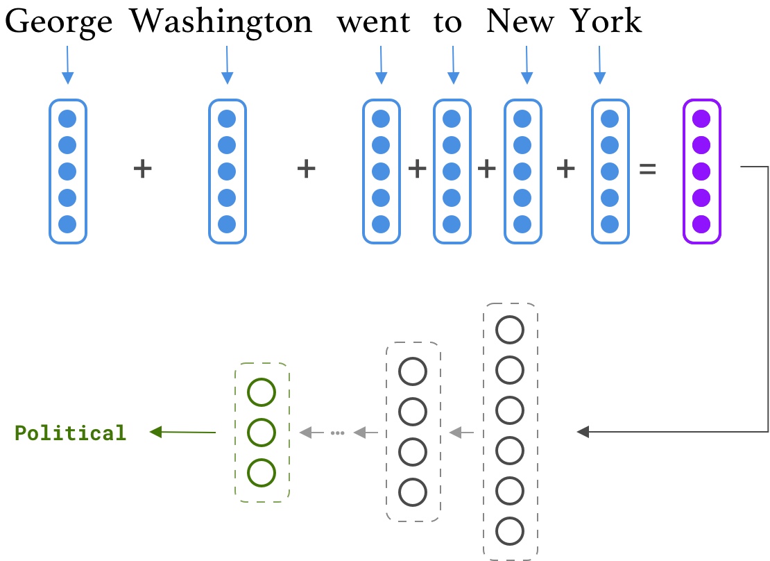
We have shown arithmetic relations are present in the embedding space. For example $e_{queen} = e_{king} + e_{women} - e_{man}$ . But are they strong enough for building a rich representation of a sentence? Can we classify a sentence according to the mean of its word's embeddings? In this section, we will find the answers to the above questions.
Assume sentence $X = [\mathbf{x^{(1)}}, ..., \mathbf{x^{(N)}}]$ is given, then a sentence representation $\mathbf{R}$ can be calculated as following:
$$ \mathbf{R} = \frac{1}{N} \sum_{i=1}^{N} e_{x^{(i)}} \ \ \mathbf{R} \in \mathbb{R}^d $$where $e_{x^{(i)}}$ is an embedding vector for the token $x^{(i)}$.
Having such a simple model will enable us to analyze and understand its capabilities more easily. In addition, we will try one of the state-of-the-art text processing tools, called Flair, which can be run on GPUs. The task is text classification on the AG News corpus, which consists of news articles from more than 2000 news sources. Our split has 110K samples for the training and 10k for the validation set. Dataset examples are labeled with 4 major labels: {World, Sports, Business, Sci/Tech}
3.1 Preprocessing
Often, datasets in NLP come with unprocessed sentences. As a deep learning expert, you should be familiar with popular text processing tools such as NLTK, Spacy, Stanford CoreNLP, and Flair. Generally, text pre-processing in deep learning includes Tokenization, Vocabulary creation, and Padding. But here we want to do one more step, NER replacement. Basically, we want to replace named entities with their corresponding tags. For example "George Washington went to New York" will be converted to "\
The purpose of this step is to reduce the size of vocabulary and support more words. This strategy is proved to be most beneficial when our dataset contains a large number of named entities, e.g. News dataset.
Most pre-processing parts are implemented for you. You only need to fill the following function. Be sure to read the Flair documentations first.
from flair.data import Token

def get_tagged_string(sentence):
  """
  Join tokens and replace named enitites
  Args:
    sentence(flair.data.Sentence): An input sentence, containing list of tokens and their NER tag

  Returns:
    output(str): A String of sentence tokens separated by spaces and
        each named enitity is replaced by its Tag

  Hint: Check out flair tutorials, https://github.com/zalandoresearch/flair/blob/master/resources/docs/TUTORIAL_2_TAGGING.md
      sentence.get_spans('ner'), sentence.tokens, token.idx and entity.tag might be helpful.
  """

  ########################################
  #     Put your implementation here     #
  ########################################

  output_toks = []

  last_end = 0
  for entity in sentence.get_spans('ner'):
    left = entity.tokens[0].idx
    right = entity.tokens[-1].idx

    output_toks += sentence[last_end: left-1]
    output_toks += [Token("<%s>"%entity.tag)]
    last_end = right

  output_toks += sentence[last_end:]

  output = ' '.join([t.text for t in output_toks])


  return output
Test your implementation:
tagger = SequenceTagger.load('ner-ontonotes')
s = Sentence('Chad asks the IMF for a loan to pay for looking after more than 100,000 refugees from conflict-torn Darfur in western Sudan.', use_tokenizer=True)
tagger.predict(s)
s_ner = get_tagged_string(s)
assert s_ner == '<PERSON> asks the <ORG> for a loan to pay for looking after <CARDINAL> refugees from conflict-torn <GPE> in western <GPE> .'
Define model's hyperparameters
VOCAB_SIZE = 10*1000
EMBEDDING_DIM = 300
NUM_CLASSES = 4
BATCH_SIZE = 512
MAX_LEN = 30
Process the entire corpus. It will approximately take 50 minutes. Please be patient. You may want to go for the next sections.
TAGGER_BATCH_SIZE = 512

if 'tagger' not in dir() or tagger is None:
  tagger = SequenceTagger.load('ner-ontonotes')

def precoess_sents(lst):
  output = []
  for i in tqdm(range(0, len(lst), TAGGER_BATCH_SIZE)):
    batch = [Sentence(x, use_tokenizer=True) for x in lst[i:i + TAGGER_BATCH_SIZE]]
    tagger.predict(batch, mini_batch_size=TAGGER_BATCH_SIZE, verbose=False)
    batch = [get_tagged_string(s).lower() for s in batch]
    output += batch

  return output

print("# Download and read dataset")
(train_sents, train_lbls), (valid_sents, valid_lbls) = read_ag_news()

print("\n# Replace named entities with their corresponding tags")
# We need to free the gpu memory due to some unknown bug in flair library
del tagger; tagger = SequenceTagger.load('ner-ontonotes')
import torch; torch.cuda.empty_cache()
train_sents_ner = precoess_sents(train_sents)
torch.cuda.empty_cache()

del tagger
tagger = SequenceTagger.load('ner-ontonotes')
torch.cuda.empty_cache()
valid_sents_ner = precoess_sents(valid_sents)
torch.cuda.empty_cache()

assert len(train_sents_ner) == len(train_lbls)
assert len(valid_sents_ner) == len(valid_lbls)

del tagger
tagger = SequenceTagger.load('ner-ontonotes')
torch.cuda.empty_cache()
del tagger

print("# Processed dataset sample")
print("train_sents[0] =", train_sents[0])
print("train_sents_ner[0] =", train_sents_ner[0])
Create the embedding matrix
# First create the vocabulary
vocab = create_vocab(train_sents_ner, VOCAB_SIZE)
tok2id = {w:i for i, w in enumerate(vocab)}

# It is a good practice to initialize out-of-vocabulary tokens
# with the embedding matrix mean
mean_embed = np.mean(np.array(list(word2vec.values())), axis=0)

# Create the embedding matrix according to the vocabulary
embedding_matrix = np.zeros((len(tok2id), EMBEDDING_DIM))
for word, i in tok2id.items():
  embedding_matrix[i] = word2vec.get(word, mean_embed)

# Fill index 0 with zero values: padding word vector
embedding_matrix[0] = np.zeros(shape=(EMBEDDING_DIM, ))
# Prepare the model input
x_train, y_train = create_model_input(train_sents_ner, tok2id, MAX_LEN), to_categorical(train_lbls, NUM_CLASSES)
x_valid, y_valid = create_model_input(valid_sents_ner, tok2id, MAX_LEN), to_categorical(valid_lbls, NUM_CLASSES)
3.2 Implementation
Let's build the model. As always Keras functional API is recommended. Numeber of layer as well as their dimensionality is totally up to you.
import keras
from keras import backend as K
class BowModel(keras.Model):
  def __init__(self):
    super(BowModel, self).__init__(name='bow')

    ########################################
    #     Put your implementation here     #
    ########################################

    self.dense_1 = Dense(128, activation='relu')
    self.dense_2 = Dense(64, activation='relu')
    self.output_layers = Dense(NUM_CLASSES, activation='softmax')

    self.embedding_layer = Embedding(
      input_dim=embedding_matrix.shape[0],
      output_dim=EMBEDDING_DIM,
      embeddings_initializer=Constant(embedding_matrix),
      input_length=MAX_LEN,
    )

  def call(self, words):
    """
    Args:
      words(Tensor): An input tensor for word ids with shape (?, MAX_LEN)
    """

    ########################################
    #     Put your implementation here     #
    ########################################

    word_embeds = self.embedding_layer(words)

    valid_words = K.sign(words)
    lengths = K.sum(valid_words, axis=1, keepdims=True)
    lengths = K.cast(lengths, 'float32')

    bow = K.sum(word_embeds, axis=1)
    bow = bow / lengths

    h = self.dense_1(bow)
    h = Dropout(0.4)(h)

    h = self.dense_2(h)
    h = Dropout(0.4)(h)

    output = self.output_layers(h)

    return output
# Let's create and visualize the NER model
bow_model = BowModel()
bow_model.compile(optimizer='rmsprop', loss='categorical_crossentropy',metrics=['acc'])
3.3 Training
# Train and visualize training
bow_model_hist = bow_model.fit(
    x_train, y_train,
    batch_size=BATCH_SIZE, epochs=10,
    validation_data=(x_valid, y_valid)
)
visualize_loss_and_acc(bow_model_hist)
bow_model.summary()
# Don't forget to run this cell.
# this is a deliverable item of your assignemnt
bow_model.save_weights(str(ASSIGNMENT_PATH / 'bow_model.h5'))
3.4 Analysis
Same as the previous section, an interactive shell is provided. You can enter an input sequence to get the predicted label. The preprocessing functions will do the tokenization, thus don't worry about the spacing.
#@title Interactive Shell
if 'tagger' not in dir() or tagger is None:
  tagger = SequenceTagger.load('ner-ontonotes')

input_text = "Chad asks the IMF for a loan to pay for looking after more than 100,000 refugees from conflict-torn Darfur in western Sudan."#@param {type:"string"}
input_sents_ner = precoess_sents([input_text])
input_tensor = create_model_input(input_sents_ner, tok2id, MAX_LEN)
pred_label = bow_model.predict(input_tensor)

print("\n-----\n\n    x: ", input_text)
print("x_ner: ", input_sents_ner[0])
print("\n   y': ", AG_NEWS_LBLS[np.argmax(pred_label[0])])
It is always helpful to see the confusion matrix:
from sklearn.metrics import classification_report, confusion_matrix

yp_valid = bow_model.predict(x_valid)
yp_valid_ids = np.argmax(yp_valid, axis=1)
y_valid_ids = np.argmax(y_valid, axis=1)
print("\n# Classification Report")
print(classification_report(y_valid_ids, yp_valid_ids, target_names=AG_NEWS_LBLS))

print("# Confusion Matrix")
cm = confusion_matrix(y_valid_ids, yp_valid_ids)
plot_confusion_matrix(cm, AG_NEWS_LBLS, normalize=False)
Obviously, this is a relatively simple model. Hence it has limited modeling capabilities; Now it's time to find its mistakes. Can you fool the model by feeding a toxic example? Can you see the bag-of-word effect in its behavior? Write down the model limitation, Answers to the above questions, and keep in mind that you need to support each of your thoughts with an input/output example
$\color{red}{\text{Write your answer here}}$
Here is some finding from our students
bellow we see effect of BOW, its seems that the correct label is business. but by avoiding relations of words and their sequence it made mistake.
    x:  American Machine and Foundry employed new 400 people
x_ner:  <org> employed new <cardinal> people

   y':  Sci/Tech
Credits: Mohammad hasan Shamgholi
4. RNN Intuition
Up to now, we've investigated window-based neural networks and the bag-of-words model. Given their simple architectures, the representation power of these models mainly relies on the pre-trained embeddings. For example, a window-based model cannot understand the previous token's label which makes it struggle in identifying multi-word entities. While, adding a single word "not" can entirely change the meaning of a sentence, the BoW model is not sensitive to this as it ignores the order and computes the average embedding (in which single words do not play big roles).
In contrast, RNNs read sentences word by word. At each step, the softmax classifier is forced to predict the label not only by using the input word but also using its context information. If we see the context information as a working memory for RNNs, it will be interesting to find what kind of information is stored in them while it parses a sentence.
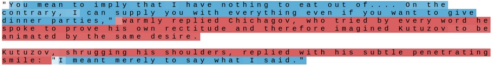
To visualize an RNN memory, we will train a language model on a huge chunk of text, and use the validation set to analyze its brain. Then, we will watch each context neuron activation to see if it shows a meaningful pattern while it goes through a sentence. The following figure illustrates a random neuron in the memory which captures the concept of line length. It gradually turns off by reach the sentence end. Probably our model uses this neuron to handle "\n" generation.
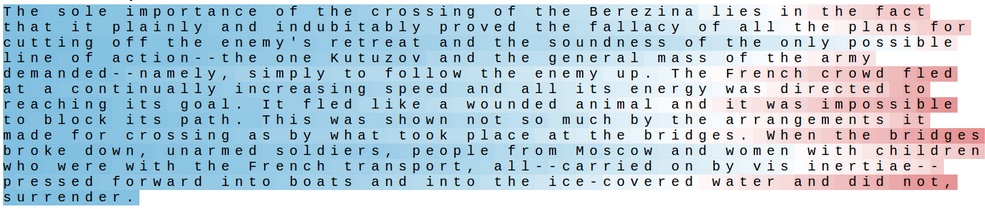
Here is another neuron which is sensitive when it's inside a quote.
Here, our goal is to find other meaningful patterns in the RNN hidden states. There is an open source library called LSTMVIs which provides pre-trained models and a great visualization tool. First, watch its tutorial and then answer the following questions:
For each model, find at least two meaningful patterns, and support your hypothesis with screenshots of LSTMVis.
$\color{red}{\text{Write your answer here}}$
Here are some patterns found by our students.
- A neuron which activates on spaces (Credits: Mohsen Tabasi)
This one is activated after seeing "a" and deactivates after reads "of"! (Credits: Mohsen Tabasi)
A combination of neurons which activate on plural nouns with ending "s"
$\color{red}{\text{Write your answer here}}$
A pattern when the model is referring to some kind of porpotion
A set of neurons which get triggered on pronouns
3- Can you spot the difference between a character-based and a word-based language model?
$\color{red}{\text{Write your answer here}}$
Char-based models have to learn the concept of word in the first place, and then they can go for much more complex pattern such as gender and grammars. However, given the fact that char-based models parse the sentence one character at a time, they can find patterns in words. i.e., They can identify frequent character n-grams in words which can help them to guess the meaning of unknown words.
References
- Erik F. Tjong Kim Sang and Fien De Meulder. 2003. Introduction to the CoNLL-2003 shared task: Language independent named entity recognition. In Proceedings of the Seventh Conference on Natural Language Learning at HLT-NAACL 2003.
- Zhang, Zhao, and LeCun, “Character-Level Convolutional Networks for Text Classification.”
- Stanford CS224d Course
- “The Unreasonable Effectiveness of Recurrent Neural Networks.” Accessed May 26, 2019. http://karpathy.github.io/2015/05/21/rnn-effectiveness/.